Constructing Excel Formulas

Constructing Excel Formulas

Understanding Basic Formula Concepts

This chapter is about building your own mathematical formulas to calculate the data on a worksheet. Formulas, and the capability to build and edit them easily, are why you would want to use an electronic spreadsheet for storing and analyzing numeric data. Even if you're a mathematical genius, allowing Excel to do your calculations saves time, reduces the margin for error, and makes updating the results fast and easy. In addition, because numbers are stored in cells and you can refer to those cells in your formulas, the process of updating formulas

with current data is automatic.

In Excel, you can write formulas from scratch or use a variety of automated features that write formulas for you. In this chapter, the focus will be on writing your own formulas to perform basic mathematical calculations in a worksheet; in Chapter 11, you'll use what you've learned about formula construction to write complex formulas that use functions to perform more intricate calculations.

There are a few basic concepts that you need to understand and remember when you write Excel formulas.

• All formulas begin with an equal sign (=).
• Formulas can use cell references and/or real numbers (called constant values) in their calculations.
• The mathematical operators Excel recognizes are + (addition), - (subtraction), * (multiplication), / (division), ^ (exponentiation), and % (percentage).
• You can add parentheses to control the order in which a formula carries out mathematical operations (when using parentheses, be sure you have complete sets of left and right parentheses).
• After a formula is entered, you'll see the formula in the Formula bar when the cell is active. The formula's result is displayed in the worksheet cell.
• When you edit a formula, you'll see the formula in both the Formula bar and the cell where you entered it, and you can edit the formula in either location.
• If you want to see all the formulas on your worksheet at once, instead of their results, you can switch the worksheet display. Press Ctrl+` (the grave accent in the upper left corner of your keyboard) to toggle between formulas and results, or click Tools, Options, and on the View tab, check the Formulas check box to show formulas (clear the check box to display results).

A formula can be as simple as =1+2. If you enter this formula into a worksheet, you'll get the result 3. But if you use cell references instead of values in your formulas, the formulas become much more flexible. For example, if you enter the value 1 in cell A1, and the value 2 in cell B1, you can write the formula =A1+B1 in any other cell, and the result will be 3. If you change the values in cells A1 and B1, the formula will continue to add the values in those cells and give you a correct result. You can build on this principle by using cell references with other mathematical operators.

For example, suppose you have a customer's invoice with a list of items and prices, and you want to add the sales tax to the subtotal. You can calculate the sales tax by multiplying the value in the subtotal cell by the sales tax. For example, in Figure 1.1, the tax rate is 5.5%, and the subtotal value is in cell E15. The formula =E15*5.5% in cell E16 calculates the correct tax whatever the subtotal.

Figure 1.1. This formula multiplies a cell reference (E15) by a constant value (5.5%).

Using AutoSum to Total Columns and Rows of Data

Because the most common worksheet calculation is the totaling of data in a list or table, Microsoft created the AutoSum toolbar button. AutoSum writes a formula that uses the SUM function to sum the values in all the cells referenced in the formula, and it writes the formula rapidly.

AutoSum attempts to guess which cells you want to use in your SUM formula. But if it guesses wrong, you can change the referenced range quickly while you enter the formula. You can use AutoSum to write quick SUM formulas using only your mouse, and you can write SUM formulas all the way across the bottom or down the side of a table in two clicks of a mouse.

To use AutoSum, follow these steps:

1. Click in the cell where you want to display the formula result.
2. Click the AutoSum button   on the Standard toolbar. Excel guesses which cells you want to include, and surrounds them with an animated border (as shown in Figure 1.2).
3. If the formula doesn't have an obvious row or column to sum, or if it guesses wrong, drag to select the cells you want to sum. The animated border surrounds all the cells you drag.
4. When the range is correct, press Enter (or click the Enter button, the green check mark left of the Formula bar) to complete the formula.

Figure 1.2. When you click AutoSum, an animated border surrounds the cells included in the formula.

If you want to write SUM formulas for several columns or rows in a table, follow these steps:

1. Drag to select all the cells that you want to display totals in, either across the bottom or down the right side of the table.
2. Click the AutoSum button. Each cell is automatically filled with a SUM formula that sums the contents of the column above it (as shown in Figure 1.3).

Figure 1.3. If you select all the cells adjacent to a table, Excel knows which cells to sum.

Editing Formulas

When you need to change a formula, either the calculation or the referenced cells, there are several techniques from which to choose: You can edit the formula in the Formula bar or in the cell.

To edit in the Formula bar, click the cell that contains the formula, and then click in the Formula bar. Use regular text-editing techniques to edit the formula-drag to select characters you want to change; then delete or type over them.  Press Enter to complete the formula. To edit the formula in the cell, double-click the cell. The cell switches to edit mode and the entire formula is visible (as shown in Figure 1.4). You can select and edit the formula just as you would in the Formula bar.

Whether you edit a formula in the Formula bar or in the cell, the references in the formula are highlighted in color, and the corresponding cell ranges on the worksheet are surrounded by borders that are color-matched to the range references in the formula, as shown in Figure 1.4. Although you can't see the actual colors in this figure, the callouts point them out, and you'll experience similar color highlights on your own screen.

Figure 1.4. Follow the colors to locate the referenced ranges.

If you need to change the cell references so the formula calculates different cells, there are several techniques you can choose from. You can type new references, click and drag a new range on the worksheet, or use range names.

NOTE: To get out of a cell without making any changes, or to undo any changes you've made before you enter them, press Esc or click the Cancel button (the red X left of the Formula bar).

Dragging Cells to Replace a Reference

A quick and direct way to add or replace a range reference is to select the range you want on the worksheet. To add a new range to the formula, click in the formula to place the insertion point where you want to add the new range reference; then use your mouse to drag and select the range you want. If you're adding a new reference to one or more existing references, type a comma to separate the references.

NOTE: To add several separate ranges all at the same time, drag to select the first range; then press and hold Ctrl while you drag to select the remaining ranges. This maneuver inserts the commas between the separate range references for you.

If you want to replace a cell or range reference, double-click the reference to highlight it in the formula (see Figure 1.5). Then click and drag the replacement cell or range on the worksheet. When you finish editing the formula, press Enter to complete the formula and close the cell.

Figure 1.5. Dragging to select range references is often more accurate than typing them.

Dragging a Range Border to Change a Reference

If you need to expand existing references (for example, if you added new columns or rows to a table and need to adjust the formula to include them), you can move or resize the colored range border to encompass the new cells. You can also move and resize the range border to reduce the range included in the formula.

To move a range border to surround different cells without changing its size, drag any side of the border. To expand or reduce the size of a range border, drag the fill handle to change the size of the range (see Figure 1.6).

Figure 1.6. You can edit a range reference by moving or resizing its colored borders.

Typing References Directly into a Formula

If you'd rather use your keyboard, you can type range references directly into the formula. Use common text-editing techniques to delete and replace characters in your references; be sure to use a colon to separate the upper-left cell reference from the lower-right cell reference in a range, and remember to separate range references with commas. If you need to reference ranges on other worksheets and other workbooks, the typing becomes a bit more complex; you'll learn about those later in this chapter, in "Referencing Other Workbooks and Worksheets."

Typing a Range Name into a Formula

If you named the ranges that you're using in formulas (a very efficient practice), you can type the range name in place of its reference.

It's useful to create range names that include some capital letters (such as Price or DecemberOrders), because the letter case will help you find misspelled range names. When you type a name into a formula, type it in all lowercase letters. If Excel recognizes the name, the characters will be converted to the case you created the name with; but if you mistype the name, the characters will remain lowercase and you'll get a #NAME? error. The lowercase name is your quickest clue to where the error is.

Pasting a Range Name into a Formula

To be sure you don't misspell a range name when you add it to a formula (or if you don't remember exactly what the range name is), you can paste it from a list of all the range names in the workbook.

To paste a name into a formula, follow these steps:

1. Click in the formula where you want to paste the name.
2. Choose Insert, Name, Paste.
3. In the Paste Name dialog box (see Figure 1.7), click the name you want and click OK.

To replace a name with another name, double-click the name in the formula to select it, and then follow the preceding steps 2 and 3 to paste a new name in its place.

If you need to change the range that's calculated in the formula, don't change the formula; instead, change the definition of the range name. Click Insert, Name, Define, and in the Define Name dialog box, click the range name. In the Refers to box, change the range references, and then click OK.

Figure 1.7. Pasting a name prevents typing mistakes.

Writing Multiple Copies of a Formula

Suppose you have a table similar to the one shown in Figure 10.8, and you need to add identical formulas at the end of each row. Instead of entering each formula individually, there are a couple of ways to create copies of your formula quickly. One method uses AutoFill to copy a formula into several more cells. Another method creates multiple copies

when you enter the formula.

Copying Formulas with AutoFill

When you copy a formula using AutoFill, each formula adjusts its references automatically so that the calculation is correct. For example, when you write a formula that sums the values in the four cells to the left (like the formula in Figure 1.8), each copy of the formula will sum the values in the four cells to its left. This works because the formula uses relative references.

To AutoFill a formula, follow these steps:

1. Enter your formula in the first cell (in this example, in the cell at the top of the column), as shown in Figure 1.8.
2. Select the formula cell. The active cell (or range) has a small black box in the lowerright corner called a fill handle.

3. Point the mouse at the fill handle; when the mouse pointer becomes a black cross, click and drag down to fill cells with copies of the formula (see Figure 1.8). You can use AutoFill to copy formulas in all four directions in your worksheet (up, down, left, and right).
4. At the end of range, release the mouse button. The cells you dragged are filled with copies of the formula, as illustrated in Figure 1.9.

Figure 1.8. When your mouse pointer is a black cross, you can drag to AutoFill the formula to adjoining cells.

Figure 1.9. When you release the mouse pointer, the cells are filled.

NOTE: You can use AutoFill to fill out a table (for example, a loan payments table) by copying an entire row or column of entries and formulas. Select the range of cells you want to copy, and drag the fill handle on the lower-right corner of the range. Also, if your table is extremely long, you can AutoFill an adjacent column by doubleclicking the fill handle instead of dragging it.

Entering Multiple Formulas All at Once

If you've already entered a formula and need to copy it across a row or down a column, AutoFill is quickest. But to enter multiple copies of a formula even faster, enter them all at the same time.

To enter the same formula in several cells at once, follow these steps:

1. Select all the cells you want to enter the formula in (see Figure 1.10). They can be in a single row or column, or in noncontiguous ranges (press Ctrl to select noncontiguous ranges).

2. Set up your formula by whatever means you normally use, but don't press Enter when you finish.

3. When the formula is complete, press Ctrl+Enter. The formula is entered in all the selected cells simultaneously (see Figure 1.11).

Figure 1.10. To enter multiple copies of a formula all at once, select all the cells first.

Figure 1.11. Press Ctrl+Enter to enter the formula in all the selected cells.

If you use range references in the formula, they'll automatically adjust to the correct references in each copy of the formula (see the section "Understanding Cell References" later in this chapter to learn more). If you use range names or worksheet labels in the formulas, each copy of the formula will find its correct range (but be careful using worksheet labels-they can be a bit unpredictable and tricky).

Using AutoCalculate for Quick Totals

Sometimes you need a quick and impermanent calculation-you need to know right nowwhat your expense account entries add up to, or how many items there are in a list. You can use AutoCalculate to get quick answers.

To use AutoCalculate, select the cells you want to calculate. The answer appears in the AutoCalculate box on the Status bar (see Figure 1.12).

Figure 1.12. Select two or more cells and see the automatic calculation of those entries displayed on the Status bar.

When you install Excel, AutoCalculate is set to calculate sums by default; but you're not limited to quick sums. You can also, for example, obtain a quick count of the items in a long product list or a quick average of your list of monthly phone bills. You can switch the calculation to Average, Count, CountNums, Max, or Min (or None to turn the feature off). To switch the calculation, right-click the Status bar (see Figure 1.13) and click the calculation you want on the shortcut menu.

Figure 1.13. Choose a different AutoCalculate function.

NOTE: AutoCalculate retains whatever function you set until you change the function again.

AutoCalculate appears in the Status bar only when two or more calculable cells are selected. For example, if the AutoCalculate function is set to Sum and you select cells that contain only text entries, AutoCalculate won't appear (because there's nothing to sum).

AutoCalculate offers the following functions:

1. Average-averages numeric values in the selected cells; ignores blank cells and nonnumeric values.
2. Count-counts all entries, whether numeric, text, or logical; ignores blank cells.
3. CountNums-counts only numeric values; ignores blank cells and nonnumeric values.
4. Max-shows the single maximum numeric value in the selected cells.
5. Min-shows the single minimum numeric value in the selected cells.
6. Sum-sums numeric values in the selected cells; ignores blank cells and nonnumeric values.

Using Arithmetic Operators for Simple Math

To perform direct mathematical operations in a formula, you use arithmetic operators. Arithmetic operators in a formula tell Excel which math operations you want to perform.

A simple formula might consist of adding, subtracting, multiplying, and dividing cells. Excel can also perform exponentiation, so you can enter a number and exponent (such as 5⁴, or 5 to the fourth power) and Excel will use the ultimate value of the exponent in the formula calculation. You can use percentages in a formula the same way-instead of entering 25% as a fractional value (25/100) or a decimal value (0.25), you can enter 25% in a formula; Excel

will calculate and use its decimal value in the math operation. Excel's arithmetic operators are detailed in Table 1.1.

Table 1.1. Arithmetic Operators

Understanding the Order in Which Excel Performs Mathematical Operations

If a formula performs more than one or two operations, you'll probably need to tell Excel in what order to perform those operations (or you may get a wrong answer).

For example, what's the answer to the equation 2+2*3? If you solve the equation left to right (perform the addition first, and then multiply), the answer is 12; but if you solve the equation using math rules (perform the multiplication first, and then the addition), the answer is 8. So how do you get Excel to solve the equation the way you want it solved, so you get the answer you want?

Excel follows standard math rules regarding which operations it performs first, next, and so forth; this is called the order of operations, and is shown as follows. To get the answer you want, you can use parentheses to divide the formula into segments and control the order of operations yourself.

• Parentheses. All calculations within parentheses are completed first.
• Negation. Making a number negative (such as -5) precedes any other operations, so that the negative value is used in the remaining calculations.
• Percent. Percentages (for example, 12%) are calculated next, so that the actual value (in this case, .12) is used in the remaining calculations.
• Exponentiation. Exponents (for example, 10^3 which means 10 cubed) are calculated next, so that the actual value is used in the remaining calculations.
• Multiplication. Performed after parenthetical operations and before all other calculations.
• Division. Follows any multiplication and is on the same level of precedence as multiplication.
• Addition. Performed after all divisions.
• Subtraction. Follows any additions and is on the same level of precedence as addition.

Controlling the Order of Operations

Even though Excel follows a set order of operations when it calculates a formula, you can alter the order in a specific formula by using parentheses to break the formula into segments. Excel will perform all operations within sets of parentheses first, and you can use this to get exactly the order of operations you want.

If multiple operations are encased in multiple sets of parentheses, the operations are performed from inside to outside, then follow the order of operations, and then left to right. Table 1.2 shows results of rearranging parentheses within the same formula. Each parenthetical calculation is performed first; then the results of those first calculations are used for the second set of calculations, which follow the order of operations. All operations on the same level (in this case, all the additions) are then performed left to right.

Table 1.2. The Results of Rearranging Parentheses

You must have balanced pairs of parentheses in any formula. If you forget a parenthesis, you'll see a message telling you there's an error. Sometimes Excel takes a guess at where you want the missing parenthesis (shown in Figure 1.14) and displays a prompt box. If the guess is right, click Yes; if it's wrong, click No and fix the formula yourself.

Figure 1.14. Excel sometimes tries to guess what you want (but it may or may not guess correctly).

NOTE: If your formula is long and contains many sets of parentheses, it can be difficult to find the missing parenthesis by eye. Instead, open the formula for editing, and use the arrow keys to move the cursor (the insertion point) through the formula one character at a time. Whenever the cursor moves over a parenthesis, both parentheses in the pair are momentarily darkened. If the parenthesis is not temporarily darkened when the cursor passes over it, that's the one that's missing a matching parenthesis for the set.

Interpreting Formula Error Messages

When something prevents a formula from calculating, you'll see an error message instead of a result. The "something" might be a reference that was deleted from the worksheet, an invalid arithmetic operation such as dividing by zero, or a formula attempting to calculate a named range that doesn't exist.

Table 1.3 lists the error messages and their probable causes (some have several probable causes, and you must do some detective work to find the problem). But Excel has tools that can help you track down the source of an error.

Locating Errors in Formulas

To locate the source of an error in a formula, begin by checking the formula itself for typing and spelling mistakes. The error may be in the formula, or it may be in a source cell that's referenced by the formula.

To locate the source of an error, follow these steps:

1. Click Tools, Auditing, Show Auditing Toolbar.
2. Click the cell containing the error.
3. On the Auditing toolbar, click the Trace Error button.

If the error originated in a source cell rather than in the active cell, tracing arrows appear and guide you visually to possible sources of error (see Figure 1.16). Blue trace lines show referenced cells, and red trace lines lead to the cell that caused the error value.

If no error-tracing arrows appear, the source of the error is in the formula itself. Use the information in Table 1.3 to find the problem.

Even if there are no errors, you can trace the dependent and precedent cells in a formula by clicking the Trace Dependents and Trace Precedents buttons. Each time you click a Trace button, tracing arrows appear for the next level of precedents or dependents.

The Remove Precedent Arrows and Remove Dependent Arrows remove the tracing arrows one level at a time.

Table 1.3. Error Values

Figure 1.16. Tracing arrows show graphically where a cell's precedents and dependents are.

Using Relative, Absolute, and Mixed Cell References in Formulas

Cells can have different types of references, depending on how you want to use them in a formula. Up until this point in the chapter, all the cell references written in the formula examples have been relative references. By default, Excel doesn't treat the cells you include in a formula as a set location. Instead, Excel considers the cells as a relative location. This type of referencing saves you from having to create the same formula over and over again. You can copy it and the cell references adjust accordingly. You saw this principle in action earlier in this chapter in the section on copying formulas ("Writing Multiple Copies of a Formula").

When writing AutoSum formulas, for example, formulas are written with relative references, and you can use AutoFill to quickly copy the formula to other cells. The copied formulas adjust themselves to the appropriate references. For example, if a relative reference in a formula refers to "the cell on my left," every copy of that formula refers to the cell on its left, no matter where you copy it.

Sometimes, however, you'll need to refer to the same specific cell on the worksheet in every copy of a formula. In a case like this, use an absolute reference. An absolute reference is fixed and never changes even if you move or copy the formula. Absolute references are denoted with dollar signs before the column and row address, such as $A$1.

For example, suppose you have a departmental budget and you like to keep a running total of what you've spent and what remains available. Figure 1.17 shows a column of running totals and a column of remaining budget dollars. The formulas use both absolute references and relative references. The formulas in the Running Total of Expenses column each sum the range from cell $C$4 to the cell left of the formula. The formulas in the Remaining Budget Dollars column each subtract the cell to the left from the Total Budget (cell $F$4). As the list of expenses in the Expenses column grows, the formulas in the Running Total and Remaining Budget columns can be quickly copied down with AutoFill.

Figure 1.17. Using absolute and relative references in the same formula enables you to create flexible lists.

On occasion, you'll need a mixed reference. Mixed references can contain both absolute and relative cell addresses, such as $A4 or C$3. For example, if you want copies of a formula to refer to the value two columns left of the formula, but always in Row 3, you'd use a mixed reference with a relative column and an absolute row (such as A$3). Copies of the formula would always refer to a value in row 3, although which cell in row 3 would depend on where the formula was.

As mentioned previously, the default reference type is always relative, which means if you click and drag cells to add references to a formula, the references will be entered as relative. If you type them, you can type the dollar signs wherever you need to designate an absolute reference, but it's faster to type relative references and then change them to absolute or mixed.

You can quickly cycle through the reference types by pressing F4 on the keyboard. For example, if a formula uses the reference A1, pressing F4 will change the reference to $A$1, A$1, $A1, and A1 (in that order) with each press. Simply stop when the reference is the type you want to use.

To change the reference type, follow these steps:

1. Double-click the cell containing the formula (or select the cell and work in the Formula bar).
2. Within the formula, click in the cell reference you want to change (see Figure 1.18).
3. Press F4 until the reference changes to the type you want. Repeatedly pressing F4 cycles through all the possible reference types.
4. Press Enter to complete the change.

Figure 1.18. To change the reference type, click in the cell reference; then, press F4.

Referencing Values in Other Worksheets and Workbooks

You can write formulas that calculate values in other worksheets and other workbooks, which is a common way to compile and summarize data from several different sources. When you write formulas that reference other worksheets and workbooks, you create links to those other worksheets and workbooks.

Referencing Other Worksheets

Suppose you have a workbook that contains separate worksheets for each division in your company. You can combine data from each division's worksheet in a Summary sheet in that same workbook to compile and analyze data for the entire company. Formulas on the Summary sheet will need to reference data on the individual Division sheets (these are called external references). You can create external references by switching to the other worksheet and clicking and dragging the cells you want to reference, just as in a same-worksheet reference; the only difference is that the cells are located on a different worksheet.

To reference data from another worksheet in your formula, follow these steps:

1. Begin building the formula.
2. When you are ready to insert the reference from another worksheet, click the tab for that worksheet.
3. Locate the cell that you want to reference, and click it. If you're referencing a range, drag across the range to select it. The sheet name and cell reference appear in the Formula bar, as shown in Figure 1.19.
4. Continue building your formula by typing the remaining operators. If your formula requires cells from other worksheets (or from the original worksheet), repeat steps 2 and 3 to add them.
5. When the formula is complete, press Enter.

Figure 1.19. An external worksheet reference is the sheet name, followed by an exclamation point, followed

by the cell reference (which can be relative or absolute).

You can also enter external worksheet references by typing them. The syntax for an external worksheet reference is

SheetName!CellReference If the sheet name contains spaces, enclose the sheet name in single quotes, like this: 'Year End Summary'!CellReference

If you change the sheet name after you've written formulas referencing it, no problem! Because they're in the same workbook, the formulas automatically update to show the current sheet name.

Referencing Other Workbooks

If you need to reference data in another workbook (called a source workbook), you can write formulas with external workbook references. For example, employees in another city send you their Excel files with operational data for their division. The following steps show how to reference two additional workbooks. To write a formula using external workbook references, follow these steps:

1. Open the workbooks you want to use, including the source workbook(s) and the workbook in which you want to write the formula, and begin building your formula.
2. Click in one of the source workbooks, and click the cell you want to include in the formula. The cell reference is added to the formula, but because it's located in another workbook, the reference includes the workbook name and worksheet name, too (see Figure 1.20). The workbook name is in square brackets and is followed by the worksheet

1. name; the worksheet name is separated from the cell reference by an exclamation point, like this: [WorkbookName]WorksheetName!CellReference
2. Continue building your formula by typing operators and clicking in other workbooks to enter the cell references.
3. Complete the formula by pressing Enter.

The formula in Figure 1.20 calculates the sum of the cells in the two source workbooks. All three workbooks are now linked by the formula.

Figure 1.20. Using multiple windows is the easiest way to work in multiple workbooks.

You can also enter external workbook references by typing them. The syntax for an external workbook reference is [BookName.xls]SheetName!CellReference If the book name or the sheet name contains spaces, enclose the entire book-and-sheet reference in single quotes, like this: '[North Division.xls]Year End Summary'!CellReference

Updating Values in Referenced Workbooks

The workbook that contains the formula is called the dependent workbook, and the workbook that contains the data being referenced is called the source workbook. If the values in the source workbooks change, the formula that references them can update its results automatically. If the source workbook is open when you open the dependent workbook, the formula is automatically updated with no questions. If the source workbook is closed when you open

the dependent workbook, you'll be asked whether you want to update all linked information (as shown in Figure 1.21).

Figure 1.21. If a workbook contains formulas that reference data in other closed workbooks, you'll be asked whether you want to update when you open the workbook.

If you click Yes, the formula is updated with current values in the source workbooks, even if those values have changed.

If you click No, the formula won't be updated with current values but will retain its previous values, which saves you time spent waiting for a large workbook to recalculate.

If the source workbook has been deleted, moved, or you changed its name, you can click No to retain the current values and rewrite the formula references, or click Yes and use the File Not Found dialog box to search for the source workbook in its new location. Searching for the file in the File Not Found dialog box is only a temporary fix; to permanently fix the link, you need to edit the links.

To edit the links in a workbook, click Edit, Links. In the Links dialog box, click Change Source. In the Change Links dialog box, locate and click the name of the moved or renamed source workbook, and click OK. Click OK to close the Links dialog box, and the link is permanently fixed (until you move the source again).

Excel in Practice

For presentation purposes, you can use Excel's auditing features to draw lines tracing references in your worksheet and then print the worksheet. The lines are printed along with the worksheet data, helping point out the connection between important data. Simply select the cell containing the formula to which you want to show the relationship of references; then display the Auditing toolbar (click Tools, Auditing, Show Auditing Toolbar). Use the Trace Precedents button to display tracing arrows. If any of the arrows obscure the view of data, enlarge the size of the row, as shown in Figure 1.22.

Figure 1.22. If you leave the tracing lines on a worksheet, they'll print to show the formula's source values.

2. Using Excel's Built-In Functions

Understanding Functions

Not all calculations are simple. Fortunately, with Excel's many functions, the program can handle just about anything you might throw its way.

Functions are built-in formulas that perform complex math for you. You enter the function name and any arguments (extra information) the function requires, and Excel performs the calculations. You saw the SUM function in action in previous chapter, "Constructing Excel Formulas," and it's a simple, straightforward function that doesn't require any further elaboration.

PMT (figures payments on a fixed-rate loan) and VLOOKUP (looks up a value in a table) are examples of common but more complex functions that I show you how to use in this chapter.

Excel comes with a slew of functions-some you use all the time, and some you'll be interested in only if you're an electrical engineer or nuclear physicist. Functions have specific names, such as SUM or AVERAGE or BETADIST, and function names must be spelled correctly or Excel won't recognize them; however, Excel provides dialog boxes that do the spelling for you and help you fill in the arguments each function requires.

Building Functions with the Paste Function Dialog Box

The easiest way to use a function in a formula is to use the Paste Function dialog box and the Formula Palette. These two integrated tools will walk you through the process of selecting and completing formulas using any of Excel's many functions. To write a formula that uses a function, follow these steps:

1. Click the cell in which you want the results of the formula to appear.
2. On the toolbar, click the Paste Function button. The Paste Function dialog box appears (shown in Figure 2.1).

Figure 2.1. The Paste Function dialog box briefly explains the selected function.

3. Click a category of functions, and then double-click the function you want to use from the list on the right. If you don't know which category to look in, click the All category and scroll through the alphabetical list of all functions. The Formula Palette opens to help you complete the function (shown in Figure 2.2).
4. Click the top argument box and read the description of the argument to figure out what information is needed. (If this is the first time you've ever used the function, click the Help button for additional information about it.)
5. If the arguments call for cell references, click or drag worksheet cells to fill in arguments. To shrink the Formula Palette so that it doesn't cover worksheet cells you want to select, click the Collapse Dialog button at the right end of the argument and select the worksheet cells. Click the Expand Dialog button (at the right end of the collapsed argument box) to redisplay the Formula Palette and continue building your function.
6. When all the necessary arguments are added, click OK. The function is built and the formula is completed.

Figure 2.2. The Formula Palette helps you fill in each argument.

This is the basic procedure for using any function in a formula. Table 2.1 describes several of the most useful Excel functions.

Table 2.1. Useful Worksheet Functions

Working with Excel's Most Useful Functions

In this section, I show you examples of the functions in Table 2.1, with suggestions for using them in real-life worksheet situations. This short list of functions contains just a few of the hundreds of functions available in Excel. If you explore the list of functions in the Paste Function dialog box, you'll find functions that calculate sine, cosine, tangent, the actual value of pi, and functions for a lot of accounting and engineering equations, logarithms, and binomials.

If you want to use complex engineering and financial functions, you'll need to install the Analysis Toolpak. Click Tools, Add-Ins, mark the Analysis Toolpak check box, and click OK.

MIN

The MIN function MIN(number1,number2,) returns the minimum, or lowest, value in a range of numbers. Of course, if your range is a single column of numbers, you can also find the smallest value by sorting or filtering the list. If your range is a large table of numbers, such as the one in Figure 2.3, the MIN function comes in handy.

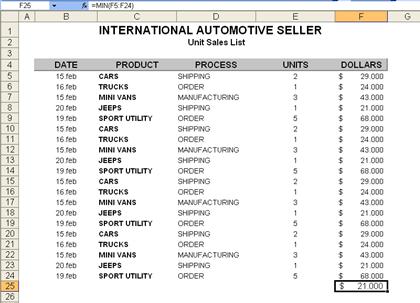
Figure 2.3. The MIN function finds the minimum value in the selected table of data.

You don't need the Formula Palette for a simple function such as MIN; to write the function yourself, follow these steps:

1. Click the cell in which you want to place the formula.
2. Type =.
3. Type min(.
4. On the worksheet, drag to select the cells you want to search for a minimum value (in this example, the range F5:F24, all the numbers in the table).
5. Type ).
6. Press Enter.

The minimum value in the worksheet table shown in Figure 2.3 is $21000, and it would have taken a bit more time to find it yourself.

NOTE: Because the minimum value is the result of a formula, it continues to find the minimum value automatically, even if you change the numbers in the table.

MAX

The MAX function MAX(number1,number2,) is the opposite of the MIN function and works exactly the same way. It finds the largest value in a selected range of cells. To write your own formula with the MAX function, you can follow the preceding procedure for the MIN function.

To write a MAX formula using the Formula Palette, follow these steps:

1. Click the cell in which you want to enter the formula.
2. Click the Paste Function button. The Paste Function dialog box appears (shown in Figure 2.4).
3. The MAX function falls under the Statistical category; click Statistical in the category list. (If you know the name of the function you want but don't know in which category to find it, click All.)

Figure 2.4. The Paste Function dialog box helps you select and write a formula using any of Excel's many functions.

4. Locate the MAX function in the function name list and double-click.
5. In the Formula Palette, highlight or delete any value in the Number1 argument text box and enter the entire table range by dragging to select the cells. In this example, the table range is F5:F24, shown in Figure 2.5.
6. Click OK.

The formula is complete, and the maximum value in the range, 68000, is displayed (see Figure 2.5).

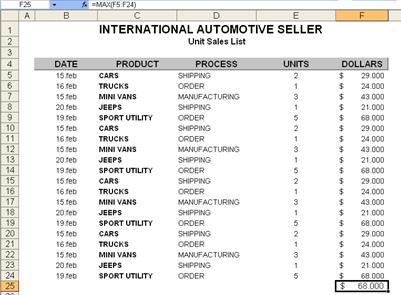
Figure 2.5. The MAX function finds the minimum value in the selected table of data.

AVERAGE

The AVERAGE function AVERAGE(number1,number2,) is another common and easy-to-use function. It's as simple to write as the SUM, MIN, and MAX functions, so it's demonstrated here without using any dialog boxes.

The important thing to know about the AVERAGE function is that it gives a more correct result than you would get by adding cells and dividing by the number of cells. If you calculate averages by adding the cells together and then dividing by the number of cells, you'll occasionally get wrong answers because if a cell doesn't have a value in it, this method averages that cell as a zero. The AVERAGE function, however, adds the cells in the selected range and then divides the sum by the number of values; so any blank cells are left out of the calculation. (The comparison is shown in Figure 2.6. Cell comments show the formulas for each cell.)

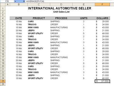
Figure 2.6. The AVERAGE function finds the minimum value in the selected table of data.

To write a formula using the AVERAGE function, follow these steps:

1. Click the cell in which you want to place the formula.

2. Type =AVERAGE(.

3. In the worksheet, drag the range of cells you want to average (or type the range name).

4. Type a closing parenthesis, ).

5. Press Enter.

SUMIF

In the worksheet table shown in Figure 2.7, I want to know how much of the product named JEEPS was sold.

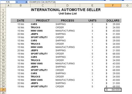
Figure 2.7. The SUMIF function finds the minimum value in the selected table of data.

To find the answer, I use a SUMIF function SUMIF(range,criteria,sum_range) which sums values if they correspond to my criteria. (In this case, I write a formula that sums values in the Total column if they correspond to the value Celebes in the Product column.) A SUMIF formula can be written in one of two ways. You can use the Formula

Palette, which is simpler and faster for single-criterion sums, or you can use the Conditional Sum Wizard, an add-in which is useful if you want to sum by two or more criteria. First, I'll show you how to write a simple SUMIF formula; then I'll show you how to use the wizard.

To use the Paste Function dialog box to write a SUMIF formula, follow these steps:

1. Click the cell in which you want to place the formula; then click the Paste Function button.
2. In the All or Math & Trig category, double-click SUMIF. The Formula Palette for SUMIF appears (see Figure 2.8).
3. In the Range box, enter the range of cells that contains the criteria (in this example, the Product column, because it contains the JEEPS criteria).
4. You can drag the cells in column C (C5:C24), or you can enter the entire column (C:C).
5. In the Criteria box, enter the criteria for which you want to sum values.

If it's a text string, as "JEEPS" is, be sure to type quotation marks around it. Alternatively, you can click a cell containing the entry JEEPS, instead of typing the text string and quotation marks.

6. In the Sum_range box, enter the range of values you want to sum (in this example, column F, entered as the range F5:F24). Your SUMIF dialog box should look similar to the one in Figure 2.9.
7. Click OK.

Figure 2.8. The Formula Palette makes the SUMIF function reasonably easy to write.

The SUMIF formula is complete. To find the total for CARS, open the cell and edit the formula. Change "JEEPS" to "CARS" and press Enter.

Figure 2.9. The SUMIF dialog box, ready to sum only JEEPS sales.

VLOOKUP and HLOOKUP

Sometimes you need to look up a value in another table. For example, in an invoice, you might want Excel to look up the state tax rate for the shipping address, or if you're a teacher keeping grade sheets, you might want Excel to look up the letter grades corresponding to your students' test score averages.

A good function for looking up values in another table is VLOOKUP VLOOKUP(lookup_value,table_array,col_index_num,range_lookup) (or its transposed equivalent, HLOOKUP)

HLOOKUP(lookup_value,table_array,row_index_num,range_lookup) These two functions are quite similar, the only difference being that one works vertically (VLOOKUP) and the other works horizontally (HLOOKUP) in the table. I'll demonstrate VLOOKUP, and when you understand VLOOKUP, you'll be able to figure out HLOOKUP if you ever need it.

Write a VLOOKUP formula.

1. Create a lookup table that contains the values you want to look up (such as a state tax rate table or the letter grades table I use in this example).

The table needs to be set up so that the values you are looking up (in this example, the test averages) are in the leftmost column (as shown in Figure 2.10) and sorted in ascending order. The table can have several columns in it, as long as the values you look up are on the left.

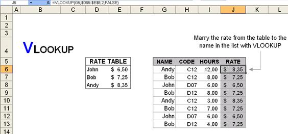
Figure 2.10. Using VLOOKUP.

For greater convenience, you can name the table and refer to it by name in the formula.

2. Click the cell in which you want the result to appear; then click the Paste Function button.

3. In the All or Lookup & Reference categories, double-click the VLOOKUP function. The VLOOKUP dialog box appears (shown in Figure 2.11).

4. Click the Lookup_value box and click the cell that contains the value you want to look up (in this case, the name ANDY).

5. Click the Table_array box and drag to select the lookup table.

6. In the Col_index_num box, type the number of the lookup table column in which Excel is to find a corresponding value. Think of the table columns as numbered left to right, starting with 1. In this example, the corresponding values (the rate) are in Column 2 of the lookup table.

7. In the Range_lookup box, decide whether you want to find the closest match or an exact match. For the closest match (which is appropriate in this case), leave the box empty. For an exact match (for example, in an unsorted list), type false.

In this case, each score you look up has a closest match, but probably not an exact match. The lookup table is sorted in ascending order, and VLOOKUP looks down the column for the closest match that's less than the test score value that it looks up. For this example, the VLOOKUP dialog box should look like the one in Figure 2.12.

8. Click OK.

The VLOOKUP function looks up the score in the lookup table, finds the closest match, and returns the rate in the second column.

Figure 2.11. The VLOOKUP dialog box is the easiest way to write the function until you become familiar with it.

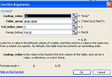
Figure 2.12. The VLOOKUP dialog box for case study.

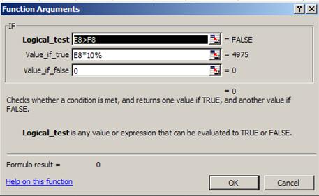
IF

The IF function IF(logical_test,value_if_true,value_if_false) is another way to determine a cell value based on criteria you set. The IF function works like this: IF a statement is true, THEN return this first value; OTHERWISE, return this second value. (Figure 2.13 shows several examples of the IF function in action.)

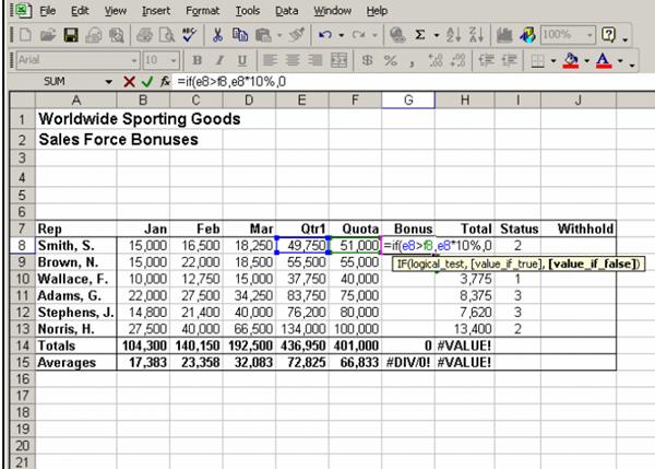
Fig. 2.13.

3. Data Management in Excel

Management of data in an Excel workbook shouldn't be time-consuming. This chapter discusses tools available within Excel that will enable you to manage both your time and data

efficiently. From extracting information with formulas, to using built-in sorting and filtering

tools created specifically for managing worksheet data and lists, to tracking changes in

worksheets shared among multiple users, Excel gives you every option necessary to effectively use your time and get the most out of your Excel data. The last section in this chapter also covers a topic close to the heart of any information manager-preventing the loss of important data by protecting workbook contents.

Using Conditional Formatting with Lists

Conditional formatting can be a great way to call out specific information within a list, or plot out timelines. The key when using conditional formats is to use a format to call out specific bits of information; for example, you can use it to call out "not to exceed" information or negative numbers. The example in Figure 3.1 uses an interactive conditional format; when a state is entered in cell D3, the conditional format highlights the cells in the list that match the entry. When you enter a project name in this cell, the conditional formatting highlights the cells referring to that project within the list. Cell E3 contains a formula that then adds the numbers in column E (the Tons column) for the highlighted list entries. The key is to use the Excel tools in innovative ways to make your everyday tasks easier. By combining conditional formatting with a formula, a single entry in cell D3 yields two results: The specified project entries are highlighted in the list, and the tonnage for that project is totaled in cell E3. You can use up to three conditional formats within a list.

Figure 3.1. By knowing how to use conditional formats, you can call out all references to the information entered in one cell.

To create an interactive conditional format, follow these steps:

1. Select the list range to which you want to apply the conditional format.

2. Choose Format, Conditional Formatting.

3. In the Conditional Formatting dialog box, choose the first condition you want. For this example, you would choose Equal To from the middle drop-down list in the dialog box, as shown in Figure 3.2.

Figure 3.2. Setting the condition.

4. In the remaining condition box, select the cell to which you want to link your condition (see Figure 3.3).

Figure 3.3. To set a link for creating an interactive conditional format, enter the cell you want linked to your list.

5. Click the Format button in the Conditional Formatting dialog box.

6. Select the desired format from the three tabs in the Format Cells dialog box. For this example, I selected black shading on the Patterns tab, and made the text bold and white on the Font tab (see Figure 3.4).

7. Click OK. The format is shown in the preview window.

8. If desired, add more criteria by clicking the Add button to add another condition.

9. Make any desired changes and then click OK.

In the sample list, when you enter a project state, the condition applies itself to the list. Any entry in the Project column that matches the value entered in cell D3 will get the conditional formatting set in the Conditional Formatting dialog box (see Figure 3.5).

Figure 3.4. Format the cells in the list that meet the conditional-formatting criteria.

Figure 3.5. When a project state is entered, the conditional format operates based on the trigger cell D3.

To understand how the formula in cell E3 works, look at the SUM(IF formula in the Formula bar in Figure 3.6.

Figure 3.6. With a simple SUM(IF formula, you can add the entries that meet the condition.

The formula sums entries in the range E6:E25 only if the nested IF statement conditions are met. The conditions are that C6:C25 is equal to D3 (that is, the project name matches the entry in cell D3). Notice that the formula appears in braces (), indicating that it's an array formula. You enter array formulas by pressing Ctrl+Shift+Enter to activate the array.

4. Using Excel to Analyze Your Data

Many Excel users input data into a worksheet, use simple functions or formulas to calculate results, and then report those results to someone else. Although this is a perfectly legitimate use of Excel, it basically turns Excel into a calculator. When you need to do more than just type data into a worksheet, you can use special Excel features to analyze your data and solve complex problems by employing variables and constraints. Goal Seek and Solver are two great tools included with Excel that you can use to analyze data and provide answers to simple or even fairly complex problems. Goal Seek is primarily used when there is one unknown variable, and Solver when there are many variables and multiple constraints. Although you may have used Solver in the past, primarily with complex tables for financial analysis, this chapter also shows you how to combine Solver with Gantt charts. Solver isn't just for financial analysis; it can be used against production, financial, marketing, and accounting models. Solver should be used when you're searching for a result and you have multiple variables that change (constraints).

The more complex the constraints, the more you need to use Solver, as shown later in this chapter for resource loading.

Both Goal Seek and Solver enable you to play "what if" with the result of a formula when you know what result you're shooting for, without manually changing the cells that are being referenced in the formula.

Using Goal Seek

The Goal Seek feature in Excel uses a single variable to find a desired result. To understand Goal Seek, let's start with a simple scenario. Suppose that you're a sales representative for a packaging business. You must achieve $100,000 in sales this year to receive a bonus. Figure 4.1 shows a table that displays the current situation-you have sold 2,000 units of a product with a per-unit sales price of $3.46. How many units must you sell to achieve your $100,000 goal?

The goal amount ($100,000 in this case) must be the result of a formula, not just plain data.

At this point, you've probably already set up the formula in your head: (100000 6920)/3.46=26901.73 units remaining to be sold. What would be the advantage of using a special Excel feature to calculate something so simple? Wouldn't you just create a formula in a cell and be done with it? The advantage of Goal Seek is that you can set up your formula just once, and then substitute different amounts to get quick alternative routes to your goal.

To use Goal Seek, select the formula cell (D7 in this example) and then choose Tools, Goal Seek to display the Goal Seek dialog box (see Figure 4.1). The following list describes the entries for each of the items in the dialog box:

Set cell specifies the location of the formula you use to get the end result. In this case, the formula is in cell D7, and simply multiplies the number of units sold by the unit price.

Type the target value in the To Value box.

In the By Changing Cell box, specify the cell location of the variable that you want to change to reach your goal-in this case, $100,000 in sales.

Figure 4.1. Specify the settings in the dialog box to begin the Goal Seek process.

As soon as you click OK or press Enter, Excel begins seeking the specified goal. In this case, the solution indicated is 28901.7341 total units at the current price of $3.46 (see Figure 4.2). In this case, you probably would need to round the solution to the nearest integer (28,902), because units aren't generally sold in fractional amounts.

Figure 4.2. Goal Seek found the desired result.

Now suppose you need to determine the unit price-the other variable in the total-sales-to date formula. If you want to sell only 2,000 units of something, how high would the price need to be for you to reach the $100,000 target? To find out, you change the By Changing Cell setting in the Goal Seek dialog box to specify cell C7, the unit price (see Figure 4.3). Here, Goal Seek will raise the price of the boxes to a dollar value that will equal $100,000 in sales but keep the units sold at 2,000. Figure 4.4 shows the outcome: To reach $100,000 by selling only 2,000 units, each unit must cost $50.

Figure 4.3. In this case, Goal Seek is adjusting the unit price to reach the target.

Figure 4.4. Finding a unit price to meet the target.

Using Solver

Goal Seek is an efficient feature for helping you reach a particular goal, but it deals with only a single variable. For most businesses, the variables are much more complex. How can you reach the profit goal if advertising expenses increase? What's the best mix of products to increase sales in the first quarter, when revenues traditionally decline for your business? Which suppliers give you the optimum combination of price and delivery? For problems like these, you can use Solver, an add-in program that comes with Excel. This powerful analysis tool uses multiple changing variables and constraints to find the optimum solution to solve a problem. Previously, Solver was a tool used primarily for financial modeling analysis; however, Solver can be used in conjunction with models of any kind that you build in Excel. Later in this section is a discussion of using Solver with Gantt charts.

NOTE: Solver isn't enabled by default. To add it to the Tools menu, choose Tools, Add-Ins, select Solver Add-in in the Add-Ins dialog box, and click OK. If asked to confirm, choose Yes. (You'll need the Office 2000 CD.)

The key to understanding complex analysis tools is to start with something relatively simple. The example in Figure 22.6 uses several variables to calculate a project's total cost. What if your total budget for the year is $500,000 (as shown in the constraints cell G20) and you were using only $375,351 (as shown in cell G16)? You want each project to have a total cost of $50,000 (G5:G14) and you want to optimize or add to your marketing and advertising dollars (columns E and F). Solver will add to the Marketing cost and Advertising cost for you, adjusting your total cost for a project to $50,000. Quite often, companies must deal with projects that have total budget caps for the year. For this, Solver works well in adjusting variables within the projects to maximize dollar amounts in certain categories, while maintaining the budget cap.

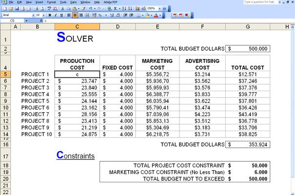
Figure 4.5. A Solver scenario where you want all projects' total costs to equal $50,000, while optimizing marketing and advertising costs.

To set up this Solver scenario, follow these steps:

1. Set up the table. In the example, the production costs are in C5:C14, the fixed costs in D5:D14, the marketing costs in E5:E14, the advertising costs in F5:F14, and the totals in G5:G14.

2. Set up the constraints. In cell G18 in the example, the constraint is $50,000 for the maximum cost per project. In cell G19, the constraint is marketing costs of no less than $6,000 per project, and the total maximum budget in cell G20 is set at $500,000.

3. Select the target cell, G16, and choose Tools, Solver.

4. In the Solver Parameters dialog box, set the parameters you want to use for the problem (see Figure 4.6). For this example, you want the target cell to be the total dollars spent (cell G16), which you want to equal the budget maximum, $500,000 (specified in the Value of box). Solver will calculate the best dispersion to achieve the optimum result by adjusting the amounts in the range E5:F14 (the changing cells).

5. Next, you add constraints to the problem. Select Add to specify the first constraint. In this example, you want to spend exactly $50,000 total on any project. The constraint cell is G18, as shown in Figure 4.7.

Figure 4.6. Establish the target cell, the target value, and the cells that can be changed.

Figure 4.7. Add variable constraints you want Solver to adhere to.

6. To add more constraints, click Add and specify the constraint. In this example, add another constraint, as shown in Figure 4.8. The marketing costs in the range E5:E14 will be greater than or equal to the constraint set in cell G19, $6,000.

Figure 4.8. The second constraint ensures that the marketing dollars allocated to each project are greater than or

equal to $6,000.

7. The last constraint is the total budget, $500,000, in cell G20 (see Figure 4.9). Don't click Add for the last constraint. Instead, when the constraints are complete, click OK to go back to the Solver Parameters dialog box. Notice that all the constraints added appear in the Subject to the Constraints list (see Figure 4.10).

Figure 4.9. The last constraint equals $500,000, or the sum of total projects.

Figure 4.10. All the constraints appear in the Subject to the Constraints list. You can add more, change, or delete any

of the constraints.

8. Click Solve or press Enter to start Solver on the problem. As Solver works, it displays a message in the status bar, as shown in Figure 4.11.

Figure 4.11. The calculations appear in the lower left while Excel runs through all the constraints set.

9. When Solver reaches a conclusion, it displays a dialog box that indicates the result and changes the specified values in the worksheet to reach the target. In Figure 4.12, notice the changed cells when Solver has created the optimum solution for the problem. The total costs now equal $500,000 and the projects all equal $50,000. 10. From here, you can save the Solver results and create an answer report that shows the original scenario of costs and the final result. Select Answer under Reports in the Solver Results dialog box, and click the Save Scenario button to display the dialog box shown in Figure 4.13.

11. If you want to reset the worksheet to return to the original values, select the Restore Original Values option to start with the original values again.

Figure 4.12. Solver enables you to create reports and save scenarios so that you can later view and recall scenarios you've run.

Figure 4.13. Name the scenario.

12. Click OK and Excel will restore the values and create the answer report (see Figure 4.14). The answer report compares the original values with the changed values and indicates the cells that were changed. This way, you can compare scenarios.

Figure 4.14. The answer report shows original values against final values, along with the category name and the adjusted cell. The target cell is called out, separated at the top.

If Solver can't reach a satisfactory conclusion with the data provided, a message box will appear. Adjust constraints or variables as needed to continue attempting to solve the problem.

Solver's solution for a complex problem may be correct but unrealistic. Be skeptical; check the appropriateness of any adjusted amounts before reporting or implementing any suggestion from Solver.

Solver can be very useful, but you don't want it to run forever attempting to solve an unsolvable problem. You can change the Solver settings before starting on the problem if you suspect that the solution may take a long time or require too much computing power.

Clicking the Options button in the Solver Parameters dialog box displays the Solver Options dialog box, in which you can set the number of iterations of the problem that Solver will run to search for an answer or the amount of time it will spend searching before giving up.