| CATEGORII DOCUMENTE |
| Bulgara | Ceha slovaca | Croata | Engleza | Estona | Finlandeza | Franceza |
| Germana | Italiana | Letona | Lituaniana | Maghiara | Olandeza | Poloneza |
| Sarba | Slovena | Spaniola | Suedeza | Turca | Ucraineana |
LONGITUDINAL
SECTIONS
Users' Manual

![]()
Innovative IT and Environmental Technologies
1.1. About Longitudinal
Sections Module. PAGEREF _Toc197328153 h
1.2. Menu Commands with
Short Descriptions. PAGEREF _Toc197328154 h
1.3. Layers PAGEREF _Toc197328155 h
2.1. Command Group: Project PAGEREF _Toc197328156 h
2.2. Command Group: Define
Axes. PAGEREF _Toc197328157 h
2.3. Command Group: Tables. PAGEREF _Toc197328158 h
2.4. Command Group: Terrain. PAGEREF _Toc197328159 h
2.5. Command: DRAW
HORIZONTAL ALIGNMENT <- AXS PAGEREF _Toc197328160 h
2.6. Command Group: Tangents
and vertical alignment PAGEREF _Toc197328161 h
2.7. Command group: Edit tangents and vertical alignment PAGEREF _Toc197328162 h
Command
Group: Roadway widths PAGEREF _Toc197328163 h
2.9. Command Group: Cross-falls. PAGEREF _Toc197328164 h
Command
group: Vertical jumps between lanes PAGEREF _Toc197328165 h
2.11. Command: Label
lanes and road edges. PAGEREF
_Toc197328166 h
2.12. Command: SAVE
LONGITUDINAL SECTION -> LS PAGEREF _Toc197328167 h
2.13. Command Group: Rehabilitation. PAGEREF _Toc197328168 h
2.14. Command Group: Quick
Volume-Calculation. PAGEREF _Toc197328169 h
2.15. Command Group: Stop
visibility length calculation PAGEREF _Toc197328170 h
2.16. Command Group: Roadway-Surface
control PAGEREF _Toc197328171 h
2.17. Command group: Road
sewer system PAGEREF _Toc197328172 h
2.18. Command group: Break
long. section. PAGEREF _Toc197328173 h
2.19. Command Group: Tools. PAGEREF _Toc197328174 h
The Longitudinal Sections module is a part of the PLATEIA software system. It is used for the longitudinal sections and vertical alignment design as a part of different engineering tasks like road and railway design, hydrology etc. This module uses terrain and axes data prepared by the Layout and Axes modules that are parts of the same software system. These data sets can be prepared in any text editor by typing of the proper data in the required format.
The Longitudinal Sections module contains a comprehensive set of commands for interactive or batch insertion of terrain lines and tangents, design of vertical alignment, calculation of superelevations based on the horizontal alignment, design of the roadway rehabilitation and fast calculation of cut and fill volumes.
A - PROJECT
Manage Project File and set System Variable.
B - DEFINE AXES
Define current axis and road category.
C - TABLES
Define, draw and edit the longitudinal section table. Together with the
set of columns required by the system, every table can include user-defined
columns.
D - SCALE SETTINGS
Set the desired vertical and horizontal scales, draw the axes system and
set the reactors.
E - TERRAIN
Draw the multiple terrain levels, save the terrain data in an
appropriate file, delete the terrain lines and exclude the points based on
distance between two points and angle difference.
F - DRAW HORIZONTAL ALIGNMENT
Define plan alignments of the road.
G - TANGENTS AND VERTICAL ALIGNMENT
Create interactive
and packet tangent, work with tables, save the tangent data and delete the
tangents. Draw the curved vertical alignment.
H - EDIT TANGENTS AND VERTICAL ALIGNMENT
Edit and delete
the vertical alignment curvature and move the curvature table.[UB1]
J - ROADWAY WIDTHS
Draw the roadway offset.
K - CROSS-FALLS
Draw the cross falls based on horizontal alignment elements, any
specific slope, label and save the cross fall data in an appropriate project
file.
L - VERTICAL JUMPS BETWEEN LANES
Define vertical jumps between lanes.
M - LABEL LANES AND ROAD EDGES
Calculate and label the lane edges.
N - SAVE LONGITUDINAL SECTION
Save the basic data that defines longitudinal section of the road in the
appropriate project file (tangents, vertical curves, minimal and maximal elevations
of vertical alignment, road edges, cross slopes, jumps and alignment elevations
in individual cross sections).
O - REHABILITATION
Manage road rehabilitation design, define the existing cross slopes,
calculate minimal elevation of vertical alignment and determine elevation
differences between old and new vertical alignment.
P - QUICK VOLUME-CALCULATION
Calculate the cut and fill volumes and draw the volume line.
Q - STOP VISIBILITY LENGTH CALCULATION
Calculate and draw stop visibility graph.
R - ROADWAY-SURFACE CONTROL
Calculate the resultant slope of a roadway and prepare the data for
drawing of the roadway contours. Enable interactive and batch insertion of
ditches, labeling and saving in the appropriate project file.
S - SEWAGE SYSTEM
Draw and label sewage system.
T - DRAW LONG. SECTION AUTOMATICALLY
The whole longitudinal section can be generated automatically based on
the date stored in a set of appropriate files.
U - BREAK LONG. SECTION
The command group is intended for preparation of longitudinal section
for plotting. Using the 31U commands, you cut longitudinal section to the
smaller sections and arrange them in a layout space.
V - TOOLS
Enable editing of the longitudinal section design by means of special
tools and utilities.
Z - UNLOAD PLATEIA LONG. SECTIONS
Unload the PLATEIA Longitudinal section menu.
This section describes the layers used by the Longitudinal Sections module. All layers are switched on by the appropriate function in real-time. The names of all the layers used by the Longitudinal Sections module start with a prefix 30_ or 31_ so they can not be confused with the layers that belong to any other program modules. You can define its own custom layers with the standard AutoCAD layer management commands.
Layer names and their short descriptions are listed in the following table:
|
Layer Name |
Layer description |
|
30_SENSOR |
sensor of the individual longitudinal section design |
|
30_TEMPLATE |
frame of the longitudinal section design |
|
30_SECTION_NAME |
code of the longitudinal section |
|
30_TABLE_NAME |
column names in longitudinal section table |
|
30_CONSTR_LINES |
different construction lines |
|
30_TERRAIN |
main terrain line |
|
30_TERRAIN_VERT |
vertical extension lines for the terrain |
|
31_TANGENTS |
tangents |
|
30_TANG_SLOPE |
schematic presentation of slopes of tangents |
|
31_VERT_ALIGNM |
vertical alignment |
|
31_VERT_CURVES |
labels of vertical curves |
|
31_AVERT_ALIGNM_LABELS |
labeling of the vertical alignment extremes |
|
30_CUT |
hatch of the cut |
|
30_FILL |
hatch of the fill |
|
31_ROAD_WIDTH_LEFT |
left road widths |
|
31_ROAD_WIDTH_RIGHT |
right road widths |
|
31_EXPANSIONS_LEFT |
left road expansions |
|
31_EXPANSIONS_RIGHT |
right road expansions |
|
31_SUPERELEV_LEFT |
cross slopes left of the centerline |
|
31_SUPERELEV_RIGHT |
cross slopes right of the centerline |
|
31_SUPERELEV_TMP |
cross slopes of the old roadway |
|
31_ROAD_EDGE_LEFT |
left edge of the roadway |
|
31_ROAD_EDGE_RIGHT |
right edge of the roadway |
|
30_VOLUME_LINE |
cut / fill volume line |
|
31_DITCH_LEFT |
ditches at the left side |
|
31_DITCH_RIGHT |
ditches at the right side |
|
31_RESULT_SLOPE |
resulting slope |
|
30_TANGENT_POINTS |
construction points of a new vertical alignment |
|
30_PLINES |
PLINE objects inserted from layout |
|
30_SYMBOLS |
symbols of intersections with utility infrastructure |
|
31_HATCH_BORDER |
vertical border lines of cut/fill hatching areas |
|
31_SUPERELEV_LEFT_1 |
left superelevation curve |
|
31_SUPERELEV_RIGHT_1 |
right superelevation curve |
Command Code: 31A
Command group Project Following comprises the following commands:
Set Project
Explore working directory
Settings
Long.Sections-Icons
Conversions
The description of the above commands can be found in the introductory part of this manual.
Command name: Reactor settings
Command code: 31A32
Icon:
Task: Switching reactors ON/OFF
Input data:
Output data:
Layers:
See also commands:
The main purpose of the Reactors is to automatically erase all the connected elements based on the selected one.
If the Reactors are switched on and you erase terrain line by using the AutoCAD ERASE command, the content of the related rubrics will be erased automatically.
Command Code: 31B
Command name: AXES-MANAGER
Command code: 31B1
Icon:

![]()
Task: Managing the projects axes: creating of a
new axis, selecting the current axis, deleting
an axis, etc.
Input data: Via dialog box
Output data: New layers (if a new axis has been defined)
Layers: This command does not use any.
See also commands: 21C1
With this command, you can manage existing axes in the drawing. Before creating a new axis, you have to define it, select its initial properties (description, station, direction, etc.) and select it as the current axis in the drawing. All AXES module commands affect only the current axis (the name of the current axis is displayed in the status line). Once the axis elements have been drawn, you can also use this command to modify the axis properties.

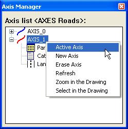
The Axes Manager dialog box explanation:
|
Active Axis |
click this button to make the selected axis the current (active) one. |
|
New Axis |
click this button to define a new axis name and its properties; when you define a new axis, new layers are created (see also Introduction: Layers). |
|
Erase Axis |
click this button to remove the axis from the drawing; when removing an axis from a drawing, the appropriate layers are removed automatically. |
|
Zoom in the drawing |
by clicking this button you can zoom to the axis. |
|
Select in the drawing |
by clicking this button you can select an axis by selecting one of its horizontal elements. |
Example:
If you erase the horizontal element of an axis, the labels of the horizontal element are erased too. To speed up global MOVE, ROTATE and similar operations, we recommend you to deactivate reactors.
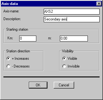
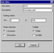
The Axis-data dialog box explanation:
|
Axis-name |
enter the name of the new axis (must not contain spaces i.e., only one word is allowed). |
|
Description |
enter an additional description of the axis (an arbitrary string). |
|
Km |
starting station in kilometers. |
|
M |
starting station in meters. |
|
Station direction |
stations of the axis can either be increasing or decreasing (stations are usually increasing, but in special cases like, e.g., watercourses stations can also be decreasing). |
|
Visibility |
specify whether the axis will be visible or invisible (if you have more than one axis, you can make one or more axes invisible). By making an axis invisible you automatically turn off all the appropriate layers (see Introduction: Layers). |
Command name: Road category
Command code: 31B2
Icon: Icon
Task: Define road category
Input data:
Output data:
Layers:
See also commands:
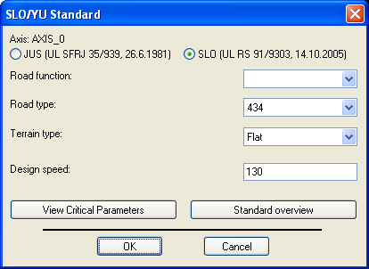
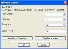
Command 31B2 is used to set up road category and terrain type. With these two parameters velocity is calculated.

 New feature in PLATEIA
is defining road category for specific axis and not for whole project. Now you
can have multiple axes with different road categories in same project.
New feature in PLATEIA
is defining road category for specific axis and not for whole project. Now you
can have multiple axes with different road categories in same project.
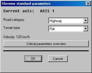

The Slovene standard parameters dialog box explanation:
|
Road category |
select among different road categories available in the selected standard, |
|
Terrain-type |
list of terrain types, |
|
Velocity |
velocity is calculated from Road category and Terrain type, |
|
Critical parameters overview |
click to open the Critical parameters overview dialogue box: |
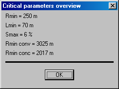
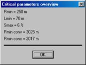
The Critical parameters overview dialog box explanation:
|
Rmin |
minimal allowed horizontal radius for curves, |
|
Lmin |
minimal allowed parameter L for spiral, |
|
Smax |
maximal allowed longitudinal level fall |
|
Rmin conv |
minimal allowed convex radius for vertical alignments, |
|
Rmin conc |
minimal allowed concave radius for vertical alignments. |

 Values
for critical parameters are checked in the following modules: Axes and
Longitudinal-sections. The program PLATEIA alerts you when some road elements contain
parameters outside the allowed range.
Values
for critical parameters are checked in the following modules: Axes and
Longitudinal-sections. The program PLATEIA alerts you when some road elements contain
parameters outside the allowed range.
Command Code: 31C
Table represents a basis for drawing of each longitudinal profile. Each drawing can contain any number of tables for drawing the longitudinal profile. PLATEIA already contains some predefined tables. User can freely customize them or create completely new ones. See commands: 31C1, 31C2, 31C3 and 31C4.
Command name: tabLeS MANAGER
Command code: 31C1
Icon:

![]()
Task: create new or edit an existing longitudinal
profile table
Input data: Via dialog box
Output data:
Layers:
See also commands: 31C2, 31C4, 31E1
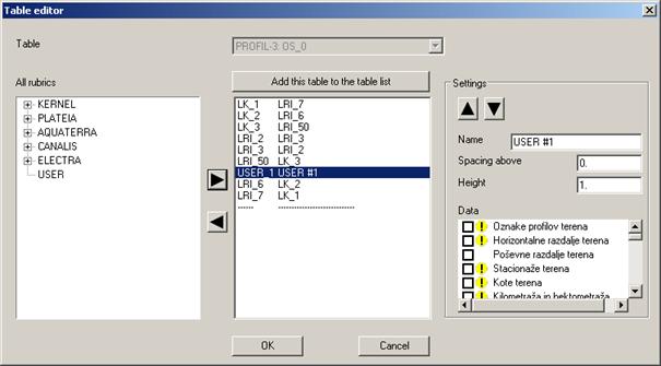
Use this command to create a new or edit an existing longitudinal profile table. The properties of the table, such as row content, row names, height etc., can be managed with this command.
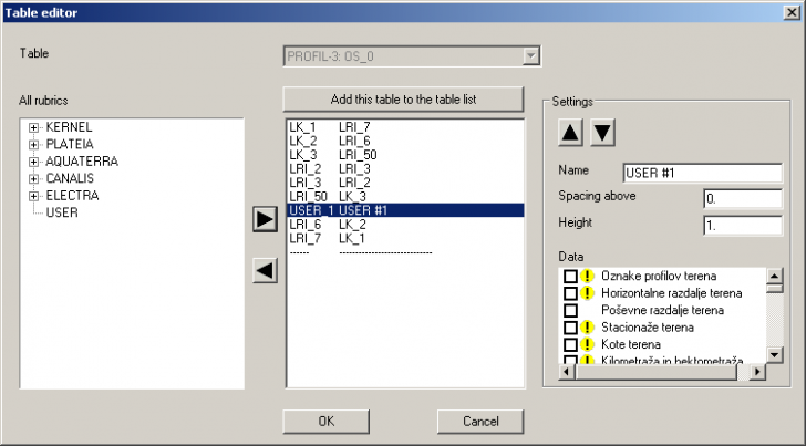
After running the command the following dialog box appears:
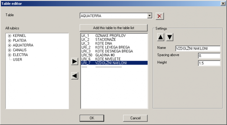
Select the table that you want to edit from the combo box on the top of
the dialog box. In the centre, the list of rows of which the table is composed
appears. Use the button

![]() to remove the selected row. To add a row,
select a rubric in the left-hand side list and click
to remove the selected row. To add a row,
select a rubric in the left-hand side list and click

![]() .
The pre-defined rows are grouped in groups, e.g. Kernel, Plateia, Aquaterra, Canalis, Electra. To add a
user-defined row, select item User.
The selected row can be added to any position in the table. The position of the
rows can also be changed later with buttons
.
The pre-defined rows are grouped in groups, e.g. Kernel, Plateia, Aquaterra, Canalis, Electra. To add a
user-defined row, select item User.
The selected row can be added to any position in the table. The position of the
rows can also be changed later with buttons

![]() and
and

![]() . In
the Settings frame, it is possible to
modify row properties: name, spacing above the row, and height.
. In
the Settings frame, it is possible to
modify row properties: name, spacing above the row, and height.
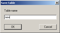
The modifications are saved by clicking the button Add this table to table list. The following dialog box will appear:
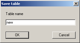
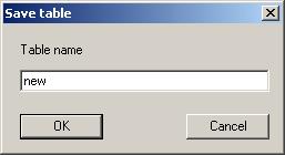
Table can be saved under a new name (in this case a new table will be created) or an existing name. These changes apply globally to all future projects.
To remove a table from the global list of tables, click the button

![]() .
.
Command name: automatic tables arrangement
Command code: 31C2
Icon:
Task: automatically
arranges longitudinal profile tables
Input data:
Output data:
Layers:
See also commands:
Use this command to automatically arrange longitudinal profile tables into rows and columns. After running the command the following prompt appears in the command line:
Number of rows for arranging sections <2>:
Enter the number of rows. Below is an example of 5 profiles before (left) and after (right) the arrangement.
Command name:
Edit current table
Command code: 31C4
Icon:
Task: edit current table in the drawing
Input data: specified in the dialog box
Output data: modified table
Layers:
See also commands: 31C1
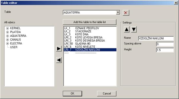
After running the command, the following dialog box appears:
In the centre, the list of rows of which the table is composed appears.
Use the button
![]() to remove the selected row. To add a row,
select a rubric in the left-hand side list and click
to remove the selected row. To add a row,
select a rubric in the left-hand side list and click
![]() .
The pre-defined rows are grouped in groups, e.g. Kernel, Plateia, Aquaterra, Canalis, Electra. To add a
user-defined row, select item User.
The selected row can be added to any position in the table. The position of the
rows can also be changed later with buttons
.
The pre-defined rows are grouped in groups, e.g. Kernel, Plateia, Aquaterra, Canalis, Electra. To add a
user-defined row, select item User.
The selected row can be added to any position in the table. The position of the
rows can also be changed later with buttons
![]() and
and
![]() . In
the Settings frame, it is possible to
modify row properties: name, spacing above the row, and height. In the Data list the list of data that can be
labelled in the selected row appears. Mark
. In
the Settings frame, it is possible to
modify row properties: name, spacing above the row, and height. In the Data list the list of data that can be
labelled in the selected row appears. Mark

![]() indicates that the data is already set to be
labelled in another row.
indicates that the data is already set to be
labelled in another row.
Also, the modifications can be saved by clicking the button Add this table to table list. The following dialog box will appear:
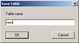
The table is saved globally and is available to the future projects.
Command name: Erase table
Command code: 31C5
Icon:
Task: Erasing of table that was drawn using the
Draw terrain command (31E1)
Input data:
Output data:
Layers:
See also commands: 31E1
Although there is an optional way of erasing a table using the AutoCAD Erase command, it is recommended that you use the 31C5 command due to reactors in a table. You can perform erasing by AutoCAD command only if you switch off the reactors in Reactor setting (31A32) command.
Command name: set number of decimal places in rubric
Command code: 31C7
Icon:
Task: Automatic changing of number decimal places
and text height in rubrics
Input data: number of decimal places, text size
Output data: modified labels
Layers: 30_RUBRIC
See also commands: 31C
This command enables automatic changing of number decimal places in rubrics. After invoking this command, the command line reads:
Select text:
Using your mouse pointer, select any text in a rubric you want to set. The following dialog box appears:
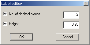
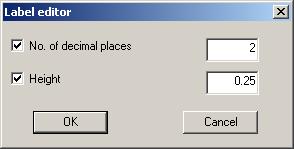
In the dialog box, one can change the number of decimal places (only active if the labels contain numeric values) and text height. All labels of the selected type will be changed.
Command name: Erase rubric content
Command code: 31C8
Icon:
Task: Erasing of rubric content
Input data:
Output data:
Layers: 30_RUBRIC
See also commands: 31C
By using the 31C8 command, you can erase content of any rubric. After invoking this command, the command line reads:
Select label:
All labels of the selected type will be erased.
Command name: Move table
Command code: 31C9
Icon:
Task: Moving of profile
Input data:
Output data:
Layers:
See also commands: 31C
Using the 31C9 command, move a profile to another position. After invoking this command, the command line reads:
Select profile element:
Select an element of the profile that you wish to move. Then move the profile to the desired location.
Command name: Set current Table
Command code: 31CA
Icon:

![]()
Task: Setting
of current longitudinal profile table for processing
Input data:
Output data:
Layers:
See also commands: 31C1
The commands of the longitudinal section module operate on the current
profile. Current profile is marked by black arrow (see figure below) in the
drawing. To select a different current profile, run this command and select an
element of the profile that you wish to become current.
Command Code: 31E
This command group contains commands for drawing and editing of the terrain lines and exporting the terrain data to the appropriate file.
The DRAW TERRAIN (31E1) command is used for inserting the main terrain line, together with any number of additional terrain lines into the current longitudinal section design.
Selected PLINE element can be saved in the terrain data file by using the Save terrain data -> LON command. The Erase terrain (31E3) command deletes the desired terrain line together with the corresponding data. By using the Filtering terrain data (31E4) command you can remove terrain points based on their distances and angle difference.
To customize the appearance of the longitudinal section design you can you can use the 31A31 command.
Command name: DRAW TERRAIN <- LON
Command code: 31E1
Icon:

![]()
Task: Drawing of the terrain line based on data
from the LON file
Input data: LON file type
Output data: terrain line
Layers: 30_TERRAIN
See also commands: 31E3, 31E4
This command reads the data from the selected LON file and inserts the appropriate terrain line.
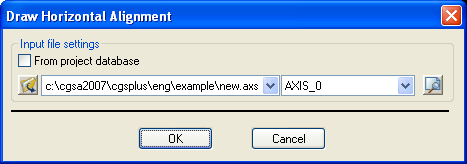
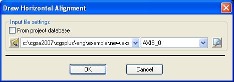
After invoking the DRAW TERRAIN <- LON (31E1) command, the DRAW TERRAIN dialog box appears:
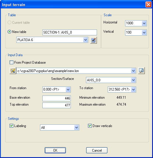
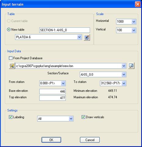
The DRAW TERRAIN dialog box explanation:
|
Table Current table |
Select this option to add terrain profile to the current table. If the terrain profile with the same name already exists in the current profile, it will be replaced. This option is only active if a profile already exists in the drawing. |
|
Table New table |
Draw terrain profile in a new table. If necessary, change the profile name in the neighbouring edit box. Select the table definition from the combo box below. |
|
|
Click this button to modify the table contents. The Table editor will appear. See command 33C4 for details. |
|
Scale Horizontal |
Select or type horizontal scale for the profile. |
|
Scale Vertical |
Select or type vertical scale for the profile. |
|
From project database |
Check to read data from the project database |
|
|
Select LON file that contains the longitudinal profile data (if From project database is not checked) by clicking on this button or select it from the list |
|
|
Click this button to view the input file in Notepad. |
|
Section/Surface |
Select section of data in selected LON file, or select surface if input is from project database |
|
From station |
Enter starting station for the profile |
|
To station |
Enter ending station for the profile |
|
Base elevation |
Enter base elevation of the plot (for main profile in the plot only) |
|
Top elevation |
Enter top elevation of the plot (for main profile in the plot only) |
|
Minimum elevation |
Minimum elevation of the section, |
|
Maximum elevation |
Maximum elevation of the section |
|
Labelling |
Check to label elevations into the table (for main profile in the table also stations and section names). Select frequency (sections all, every second ) of labelling from the list. |
|
Draw verticals |
Check to draw verticals from section nodes. |
|
Rubric |
Select row into which elevations will be labelled. This option only appears for additional profiles. To use this option, insert a user row into the table. Main profile elevations are labelled into the predefined row (TERRAIN ELEVATION). |
The profile
station can either increase or decrease. The latter option is compatible with
the increasing flow direction for the rivers. The profile station direction is
controlled with the selection of From station and To station fields. If you
want the profile station to increase, From station must be less than To
station. If you want the profile station to decrease, From station must be
grater than To station.
The record that describes every terrain point has the following structure :
STA_KM STA_M ELEV PROF
Fields description:
STA_KM station in kilometers (INTEGER),
STA_M station in meters (REAL),
ELEV point altitude, point elevation (REAL),
PROF profile code (STRING).
LON file type can contain the following special characters:
Comment,
# SECTION start
of the new section of data followed by the SECTION
name,
Example of the LON file:
# BASE TERRAIN
* test data for the terrain
250 234.45 a1
250.5 234.34 a2
60.0 235.2 0
# OLD ROAD
* test data for the terrain
250 234.65 a1
250.5 234.54 a2
60.0 235.4 0
Command name: Save terrain data -> LON
Command code: 31E2
Icon:
Task: Saving of the PLINE object in the terrain file
Input data: Via dialog box
Output data:
Layers:
See also commands:
By using the Save terrain data -> LON command you can save the data for the existing terrain or selected PLINE object. If you save the existing terrain, the file will contain the profile codes for the selected terrain line. As PLINE does not contain point codes, program will add code 0 for all the points.
After invoking the Save terrain data -> LON command the following dialog box appears:
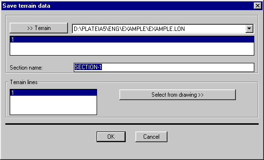
The Save terrain data dialog box explanation:
|
Terrain |
insert/choose the terrain filename here (LON), |
|
Section name |
insert the name of the section of data, |
|
Terrain lines |
shows the list of the terrain lines in the current drawing, |
|
Select from drawing |
enables selecting the terrain line form the drawing. |
Points will be saved in the following format:
STA_KM STA_M ELEV PROF
Fields description:
STA_KM station in kilometers (INTEGER),
STA_M station in meters (REAL),
ELEV point altitude, point elevation (REAL),
PROF profile code (STRING).
Lines of the file type LON can also start with the following special characters:
Comment,
# SECTION start of the new section of data followed by the SECTION name,
Example of the LON file:
# BASE TERRAIN
* test data for the terrain
250 234.45 a1
250.5 234.34 a2
60.0 235.2 0
# OLD ROAD
* test data for the terrain
250 234.65 a1
250.5 234.54 a2
60.0 235.4 0
Command name: Erase terrain
Command code: 31E3
Icon:
Task: Deleting the terrain line and the content
of corresponding rubrics
Input data:
Output data:
Layers:
See also commands:
This command enables erasing the selected terrain line together with the content of the corresponding rubrics (PROFILE CODES, STATIONS and ELEVATIONS). If the Reactors are turned on (See 31D command), terrain line can be deleted by using the AutoCAD ERASE command. The contents of all the corresponding rubrics will also be deleted.
Command name: Filtering terrain data
Command code: 31E4
Icon:
Task: Straightening of the terrain line based on
distance and angle tolerance
Input data: Via dialog box
Output data:
Layers:
See also commands:
You can reduce the number of short segments that are part of the terrain line by using the Filtering terrain data (31E4) command. Clean up of the terrain line is based on the distance between two points and/or the elevation difference between three consecutive points.
Points will be excluded from the terrain line in the following cases:
a. When the distance between two neighboring points is less than the tolerance set in the dialog box and
b. When the angle between three consecutive points is less than the tolerance set in the dialog box.
The Filtering terrain data dialog box shown below appears after invoking the 31E4 command. It is used for the selection of clean up method and setting of distance and angle tolerances.
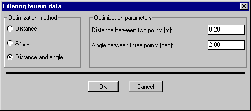
Figure: Way of extracting points from the terrain line based on a distance between the two points.
The figure above shows the way of extracting points from the terrain line based on a distance between the two points. d1 distance is less than the defined tolerance, so T1 point is extracted from the terrain line which is straightened by joining points T0 and T2 (shown as dashed line).
Figure: Way of extracting points from the terrain line based on a elevation difference between three consecutive points.
The figure above shows the way of extracting points from the terrain line based on a elevation difference between three consecutive points. The k1 angle is less than the defined tolerance, so T1 point is extracted from the line. The terrain line is straightened by means of the segment shown as dashed line.
Command Code: 31F
Command name: DRAW HORIZONTAL ALIGNMENT <- AXS
Command code:
Icon:

![]()
Task: Creates schematic drawing of horizontal
road elements
Input data: Via dialog box
Output data:
Layers:
See also commands:
The DRAW HORIZONTAL ALIGNMENT <- AXS command inserts a number of horizontal and inclined lines in the Horizontal elements rubrics creating a schematic overview of horizontal alignment centerline (lines, transitions and partial transitions).
In addition to the aforementioned lines, program will insert values for the following parameters:
length for linear element,
parameter A and curve length for transitions and partial transitions,
radius and curve length for arc element.
Horizontal alignment is very important for the calculation of roadway slopes.
You can customize the appearance of horizontal alignment by setting the variables (31A31).
Terrain line has to be inserted in the longitudinal section design before the Horizontal alignment elements. Schematic overview of the horizontal alignment is generated based on the data stored in the appropriate AXS file that can be created by the 2E5 command.
Every horizontal alignment element is defined by the data structure of five consecutive lines with described below:
NO TYPE OZ_NO_E ST_STAT ST_R Y_ST_POINT X_ST_POINT ST_DIR_ANG 1
A LENGTH END_R Y_END_POINT X_END_POINT CHG_ANG 2
END_STAT Y_PRE_TAN X_PRE_TAN END_DIR_ANG 3
Y_CEN_POINT X_CEN_POINT TANGENT1 4
Y_MID_TOC X_MID_POINT TANGENT2 5
Codes explanation:
NO ordinal number of the element in the horizontal alignment (INTEGER),
TYPE type of the horizontal alignment element (STRING),
O_NO_E ordinal number of the element (INTEGER),
ST_STAT starting station of the element (REAL),
ST_R starting radius of the element (REAL),
Y_ST_POINT Y coordinate of the start point (REAL),
X_ST_POINT X coordinate of the start point (REAL),
ST_DIR_ANG starting direction angle (REAL),
abel of the first line in the element data structure (INTEGER),
A parameter A of the transition (REAL),
LENGTH length of the element (REAL),
END_R ending radius of the element (REAL),
Y_END_POINT Y coordinate of the end point (REAL),
X_END_POINT X coordinate of the end point (REAL),
CHG_ANG change of the direction angle (REAL),
label of the second line in the element data structure (INTEGER),
END_STAT ending station of the element (REAL),
_INT_TAN Y coordinate of the intersection of tangents (REAL),
_INT_TAN X coordinate of the intersection of tangents (REAL),
END_DIR_ANG ending direction angle (REAL),
label of the third line in the element data structure (INTEGER),
Y_CEN_POINT Y coordinate of the center point (REAL),
X_CEN_POINT X coordinate of the center point (REAL),
TANGENT1 length of the left tangent (REAL),
label of the fourth line in the element data structure (INTEGER),
Y_MID_POINT Y coordinate of the mid point (REAL),
X_MID_POINT X coordinate of the mid point (REAL),
TANGENT2 length of the right tangent (REAL),
label of the fifth line in the element data structure (INTEGER).
AXS file type lines can also start with the following special characters:
Comment,
# SECTION start of the new section of data followed by the SECTION name,
Example of the AXS file:
# FIRST AXES
* NO TYPE OZ_NO_E ST_STAT ST_R Y_ST_POINT X_ST_POINT ST_DIR_ANG 1
A LENGTH END_R Y_END_POINT X_END_POINT CHG_ANG 2
END_STAT Y_PRE_TAN X_PRE_TAN END_DIR_ANG 3
Y_CEN_POINT X_CEN_POINT TANGENT1 4
Y_MID_TOC X_MID_POINT TANGENT2 5
1 LINE 1 0.0 00 NESK -6.053 226.943 48d0'15' 1
139.872 NESK 97.90 0 320.529 2
139.872 3
4
5
2 TRANSITION 1 139.872 NESK 97.90 0 320.529 48d0'15' 1
101.296 102.610 +10 0.0 00 183.697 374.601 29d23'44' 2
242.482 149.461 366.948 77d23'59' 3
205.512 277.0 09 69.378 4
35.082 5
3 CIRCULAR_ARC 1 242.482 +10 0.0 00 183.697 374.601 77d23'59' 1
197.517 +10 0.0 00 303.816 258.668 1131E10'8' 2
439.999 331.615 407.665 190d34'7' 3
205.512 277.0 09 151.568 4
274.958 348.962 151.568 5
* Total length of the alignment: 439.999
* Curvature characteristic: 0.1
After invoking the DRAW HORIZONTAL
ALIGNMENT <- AXS (
The distance of the horizontal alignment breaking points from the inserted centerline indicates the ratio between radii of circular arcs and transitions (see Figure).
![]()
Figure: Horizontal alignment.
[l2] Command Code: 31G
When iserting tangents, you can modify the plan appearance by setting the following parameters:
[310501] Tangents-line color (4),
[310502] Tangents-line-type (CONTINUOUS),
[310503] Vertical lines for labeling tangents color (1),
[310504] Vertex-symbol for labeling tangents color (9),
[310505] Inclined lines for labeling tangents color (1),
[310506] Tangent-label text-color (1),
[310507] Tangent-label text-height (0.2),
[310508] Number of decimal places for labeling tangent slope (4),
[310509] No. of decimal places for saving station and elevation to TAN file. (10).
[310510] tangent circle radius, when labelling tangents[l3]
Layers: 31_TANGENTS, 31_VERT_ALIGNM
See also commands: 31G2 -31G7
If there is already a drawn tangent, this command first offers either an option of drawing of an existing tangent or a new one.
Tangents can be inserted to longitudinal section by selecting of vertex points by means of a mouse. Alternatively, they can be inserted by selecting parameters in a dialog box that appear after definition of the first tangent point in drawing. In the first example, user can barely control their values while in the second one user can precisely define the next vertex point position.
You can select only two parametres at a time. They can be fixed at certain value or they change by a preset step. If both are fixed, also point in drawing is completely defined and cannot be moved by the mouse. It can be only confirmed or settings may be changed.
Using the Draw tangents dialog box, you can select the following parameters:
station
elevation/height
distance tangent length
slope
section
Using the Step settings option, set individual value change step instead of exact parameter value. This function resembles the Snap and Polar AutoCAD options.
You can define these parameters already when drawing tangents using the Curve Parameters dialog box. Or, you can define tangent changes and their modification for later editing using the Change Vertical Curve (31H5) command.
For explanation of individual parameters see the Change Vertical Curve (31H5) command.
Prior to interactive tangent insertion, select construction points in drawing through which a vertical alignment should go. Input construction points using the Define station and elevation, draw point (31V6) command.

The upper drawing shows a preview of vertical curve based on the next tangent selected parameters (position definition).
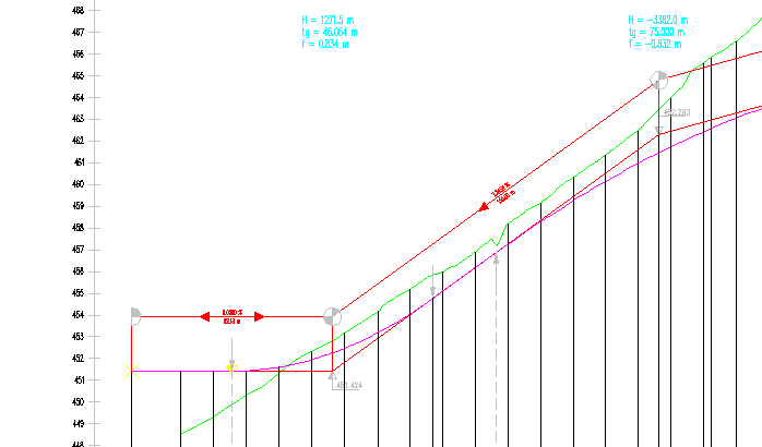
Drawing and labeling of vertical alignment after you have finished a tangent definition.
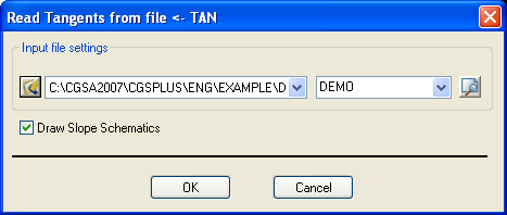
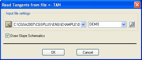
Command name: Read tangents from file <-TAN
Command code: 31G2
Icon:
Task: Inserting of tangent and vertical alignment
from file
Input data: TAN
file
Output data: drawn
tangents and vertical alignment
Layers: 31_TANGENTS, 31_VERT_ALIGNM
See also commands: 31GA
The Read tangents from file <-TAN (31G2) command is the second way of inserting tangents to a longitudinal section. Data that define tangents can be previously prepared and stored in a TAN file type for section of any length. Each vertex point is defined by the following line form:
STA_KM STA_M HEIGHT [RADIUS]
or
STA_KM STA_M HEIGHT [RADIUS] [LABEL]
Both ways of inserting tangents are allowed. Second form is an updated version of the first one where a numerical label of individual vertex is additionally recorded. Numerical vertex labels are needed in order to assure a uniform tangent-vertex labelling in case of automatical drawing of longitudinal section using the 31T command or when you want to draw only one section from the TAN file.
Codes description:
STA_KM station in kilometers (INTEGER),
STA_M station in meters (REAL),
HEIGHT point altitude, elevation (REAL),
[RADIUS] curvature radius (REAL). In case of the first TAN file form, radius value does not necessarily get outputted. In the case of the second TAN file form when vertical curve is not defined, the NULL string gets outputted.
[LABEL] Vertical curve label is a vertex number. The first and and the last vertex carry a 0 label while vertices in between carry numerical labels.
Brackets in the upper line ([]) stand for an optional parameter which can exist or not. The RADIUS parameter is used when saving a curvature radius using the Read tangents from file <-TAN (31G2) command.
TAN file type lines can also start with the following special characters:
* star in the first column stands for comment or comment line,
# SECTION start of the new section of data followed by the SECTION name,
# AXS_0
*! STA_KM STA_M HEIGHT RADIUS LABEL
0 980.4494881956 238.9757059145 NULL 0
1 734.6050172909 196.7623468127 15260.947 1
3 448.5948537498 185.5237253988 24568.893 2
4 114.99410 06061 199.2293615589 NULL 0
Tangents are inserted on the 31_TANGENTS layer as one single PLINE object over the whole processed longitudinal section.
[l5] Command
name: Convert PLINE to tangent
Command code: 31G3
Icon:

![]()
Task: Converting any polyline to tangent
Input data: Polyline
Output data: Tangents and vertical alignment
Layers: 31_TANGENTS, 31_VERT_ALIGNM
See also commands: Command group 31G

 This
command enables drawing of a tangent over any polyline. Polyline can be drawn
using either any AutoCAD command or some other program. Using the 31G3 command,
you can convert a selected polyline into a PLATEIA tangent that can be used in
the rest of PLATEIA functions working with tangents.
This
command enables drawing of a tangent over any polyline. Polyline can be drawn
using either any AutoCAD command or some other program. Using the 31G3 command,
you can convert a selected polyline into a PLATEIA tangent that can be used in
the rest of PLATEIA functions working with tangents.
After invoking the command, you need to select a polyline to be converted into tangent. Command line reads:
Select polyline:
After selecting a polyline, a dialog box with options opens. Parameters can be edited later using theConvert pline to vertical alignment (31H5) command.
If tangent already exists, program prompts you and offers possibility to erase it.
Command name: CALCULATE AND LABEL TANGENTS
Command code: 31G4
Icon:

![]()
Task: Schematic labeling of tangents
Input data:
Output data:
Layers: _TANGENTS
See also commands: 31G1, 31G2
Using the Label settings (31G4) command, you can switch off labeling of tangents. You can separately define labeling and drawing of tangent elements:
in the highest and lowest point,
cut and fill surfaces,
startings and endings of main elements,
equidistantly at selected distance.
Tangents can be edited by using standard AutoCAD commands such as PEDIT, STRETCH or grip editing. This way you can move vertices, add new or remove some of the existing ones.
 When editing tangents by using AutoCAD commands,
values in the tables are not updated automatically. To update these values, you
have to use the (31G4) command. After invoking the command, you need to select
a point of schematic labeling of tangents or confirm it by ENTER. In order to
draw an vertical alignment properly, save updated tangent values to the TAN
file.
When editing tangents by using AutoCAD commands,
values in the tables are not updated automatically. To update these values, you
have to use the (31G4) command. After invoking the command, you need to select
a point of schematic labeling of tangents or confirm it by ENTER. In order to
draw an vertical alignment properly, save updated tangent values to the TAN
file.
Command name: Define boundary for coloring cuts and fills
Command code: 31G5
Icon: None.
Task: Defining of boundary for coloring cut and
fills
Input data: Drawn vertical lines using the Line command
on any layer
Output data: Boundary vertical lines on the
31_HATCH_BORDER layer
Layers: 31_HATCH_BORDER
See also commands: 31G
The Label settings (31G4) command comprises an option for appropriate coloring of cut and fill areas (between terrain and vertical alignment). This may be of obstructive nature in the case of bridges, tunnels and similar features. To avoid the problem, use the Define boundary for coloring cuts and fills (31G5) command.
First draw two vertical lines in a longitudinal section drawing. Use AutoCAD LINE command on any layer or the Auxiliary lines (31V4) command. Vertical lines should represent the start and end of area that will not be colored. Then use the Define boundary for coloring cuts and fills (31G5) command to convert selected lines to the border ones on the 31_HATCH_BORDER layer. If you proceed with the Label settings (31G4) command and select area coloring, areas between border lines stay uncolored.

An individual longitudinal section can comprise any number of areas for which cut and fill areas will not be colored.
[l8] Command
name: erase tangents and vertical
alignment
Command code 31G6
Icon: None
Task: Erasing of tangents, vertical alignment and
related rubric contents
Input data: selected
tangents
Output data: erased
selected data
Layers: 31_TANGENTS, 31_VERT_ALIGNM
See also commands: 31G1, 31G2, 31G8
The Erase tangents and vertical alignment (31G6) command enables a simple erasing of all tangent and vertical alignment elements and related rubrics (LONGITUDINAL SLOPES, ALIGNMENT ELEVATION, etc.). Erasing of tangents and vertical alignment can be used when you want to perform certain modifications on vertical alignments which cannot be done using the commands from the Edit tangents and Vertical Alignment (31H) command group. When this is the case, erase the existing tangent and construct a new one. After invoking the command, select a tangent to be erased and confirm your selection.
Command name: Save tangents And vertical alignment to file
-> TAN
[l10] Command code: 31G7
Icon:
Task: Saving tangents to file
Input data: Via dialog box
Output data:
Layers:
See also commands: 31G2
By using this command you can save the data that define the vertices of tangents and vertical alignment radius. Usually you use it in combination with the Read tangents from file <- TAN (31G2) command. One single TAN file can contain data defining different version of tangents of one or several axes that can later be inserted in the longitudinal section. Program saves tangent data to the file having the following form:
STA_KM STA_M HEIGHT [RADIUS] [LABEL]
Codes description:
STA_KM station in km (INTEGER),
STA_M station in m (REAL),
HEIGHT elevation, label (REAL),
[RADIUS] column for later insertion of curvature radius,
[LABEL] numerated vertex label (for example 0,1,2,3, etc.) First and last vertex on tangent are labeled 0.
TAN file type lines can also start with the following special characters:
* star in first column stands for comment or comment line,
# SECTION start of the new section of data followed by the SECTION name.
# AXS_1
*! STA_KM STA_M HEIGHT RADIUS LABEL
0 998.1106577605 230.0456606244 NULL 0
2 83.8239166035 190.5832682366 30 029.022 1
3 570.8549729964 190.2984881058 12920.535 2
4 98.2014160155 211.7209298492 NULL 0
[l12] Command code: 31H
The Vertical Alignment (31H) command group contains commands for interactive design and labelling of vertical alignment. You can edit vertical alignment by using one of the following commands:
Edit geometry (31H1),
Change vertical curve (31H5),
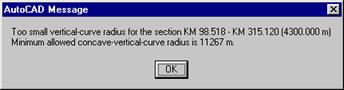
Vertical curve radius size can be checked according to a selected calculation standard in the Road category (31B2) command. You can set the checking switch on/off using the Variable setting (31A31) command (parameter [310 001]) Check vertical element by calculation standard (1-Yes, 0-No). If longitudinal slope of tangent and vertical curve exceed allowed values, program prompts you by the following windows:

When saving vertical curves, you can modify a plan appearance by setting of the following parameters:
[310301] Vertical curve labeling style (111111111)
This parameter consists of nine digits. Every digit can be evaluated as 0 or 1.
Value 0 is equal to off and value 1
to on. Meaning of these nine digits
is as follows:
1st Digit: labelling of curve codes,
2nd Digit: labelling of curve radiuses,
31Td Digit: labelling of slope change,
4th Digit: labelling of tangent length,
5th Digit: labelling of parameter A,
6th Digit: labelling of station of vertex,
7th Digit: labelling of vertex height,
8th Digit: labelling of curve length and
9th Digit: drawing of a table border.
[310302] Vertical curve vertex-density (40)
Vertical alignment curves are circular arcs that are represented as parabolas
according to the horizontal and vertical scale setting (eg. 10 00/10 0). In the
drawing, these curves are approximated with short line segments (chords). The
accuracy of presentation depends on the setting of this parameter. The default
value of 40 vertices usually gives a sufficient accuracy.
[310303] Vertical curve station-labelling style (1)
You can label the stations in three different display formats as follows:
format 1234.56 parameter value 1,
format 1+234.56 parameter value 2,
format 1.2+34.56 parameter value 3.
[310304] Vertical curve label text-color (2),
[310305] Vertical curve number-label text-color (4),
[310306] Vertical curve radius-label text-color (1),
[310317] Vertical-alignment label-frame color (7),
[310313] Vertical-line for vertical-curve-labels color (7),
[310314] Vertical-line for vertical-curve-labels type (LK_HIDDEN),
[310315] Vertical alignment elevation-label text-height (0.25),
[310316] Vertical alignment elevation-label text-alignment (_M),
[310317] Vertical alignment elevation-label text-color (_BYLAYER),
[310318] Vertical-alignment-curve color (6),
[310319] Vertical-alignment-curve linetype (CONTINUOUS),
[310320] Scale-factor for automatic vertical-curve
generation (0-10 0) (50).
When generating the vertical-curve automatically, program determines the
biggest possible radius for every single vertex. By setting the scale factor
you can define the actual size of a radius that will be inserted in every
vertex. Value of 50 means that in every vertex the radius will be one half of
its maximum size.
[310321] Rounding values for vertical-curves radius
(10 0, 10 00, 250 0 ) (10 0)
In the process of an automatic vertical alignment generating, the values of
calculated radii multiplied by factor are rounded to the desired rounding
value. To round these values to
[310322] Vertical curve type (0-arc, 1-parabola)
When performing an automatic save of the vertical curve, maximum radius that is calculated and multiplied by factor rounds to a desired value. For rounding radius at 10 0m, enter value 10 0.
Figure: Constructed vertical curves.
Vertical alignment of a road profile is constructed based on tangents and other curvature parameters such as:
point above/bellow the vertex,
distance between vertex and curve,
radius,
tangent length
selected point on a curve.
 Vertical
alignment is constructed by drawing the curves only. Curves can be drawn in any
desired order. When labelling the vertical alignment, the linear segments are
inserted automatically. Vertical alignment consists of two types of elements:
lines and curves. Every element is represented by a single PLINE object.
Vertical
alignment is constructed by drawing the curves only. Curves can be drawn in any
desired order. When labelling the vertical alignment, the linear segments are
inserted automatically. Vertical alignment consists of two types of elements:
lines and curves. Every element is represented by a single PLINE object.
Using the Edit geometry (31H1) command, you can change geometry of the drawn tangents. After invoking the command, select a vertex to be edited. After selecting it, a dialog box opens in which vertex parameters may be changed.
Station
Height
Length
Slope
Section
Active vertex is marked with a red circle.
The same as with the Draw tangents (31G1) command, user can set a step for changes that will be considered when defining new tangent value in drawing. Parameter changes can be checked by preview simply by clicking Refresh. If no parameter is defined, you can move tangent vertex freely.
New tangent vertex position can be defined also by clicking Jig. After invoking the command, dialog box closes and you can define a new point position in drawing. Whenever a change takes place, tangents and a vertical alignment get refreshed and attributed values drawn.
Using the Previous and Next buttons, you can move through individual vertices in drawing without leaving the dialog box.
Parameter description related to an individual tangent vertex:
|
Station |
Station value |
|
H (m) |
Height |
|
L (m) |
Length |
|
S (%) |
Tangent slope |
|
Step |
Step by which parameters values change |
|
Refresh |
Refresh drawing |
|
> |
Element selection direction in drawing (> right, < left) |
|
Section |
Section name |
|
Section + |
Offset from section in m |
|
Step setting |
Parameter change step setting |
|
|
Erase vertex |
|
|
Add vertex |
|
>> |
Define a new vertex position in drawing |
|
Previous |
Active vertex move to the previous one |
|
Next |
Active vertex move to the next one |
The methods of vertical alignment curve definition are shown below
Commmand name: MOVE TANGENT-VERTEX
Command code: 31H2
Icon:

![]()
Task: Tangent vertex reposition
Input data: Selected vertex, newly selected vertex
location
Output data:
Layers: 31_TANGENTS, 31_VERT_ALIGNM
See also commands: 31G1, 31H1, 31H3, 31H4, 31H1
This command enables a desired tangent vertex move. After invoking the command, only tangent is visible due to better visibility. Command line reads:
Select vertex on tangent:
Using the mouse pointer, select a vertex to be moved. After selecting the vertex, you can have a preview of the new tangent and vertical alignment position. After defining the new position, all corresponding elements will be drawn in section.
Command name: INSERT NEW TANGENT-VERTEX
Command code: 31H3
Icon: None
Task: Inserting new tangent-vertex in desired
point of the existing tangent
Input data: Existing tangent
Output data: New tangent with new vertex
Layers: 31_TANGENTS, 31_VERT_ALIGNM
See also commands: 31G8
When you want to insert a new vertex in existing tangent, you use the Insert new tangent vertex (31H3) command. This command, similarly to option Edit vertex, Insert associated with the AutoCAD command PEDIT, inserts a new vertex to the selected point on tangent. At the same time, the 31H3 command updates labels for the slopes and lengths of tangents.
 This command functions very similarly
to the one used for a vertex reposition. You can have a preview showing a new
tangent and vertical alignment position. Prior to inserting the vertex to a
selected position, you can define a construction point using the Define station and
elevation, draw point (31V6) command.
This command functions very similarly
to the one used for a vertex reposition. You can have a preview showing a new
tangent and vertical alignment position. Prior to inserting the vertex to a
selected position, you can define a construction point using the Define station and
elevation, draw point (31V6) command.
Insertion of a new vertex can be alternatively done by saving of existing tangents to the TAN file using the Insert new tangent vertex (31G7) command. Then you need to insert a new line representing a new vertex to the TAN file and then read new tangents using the Read tangents from file <-TAN (31G2) command.
Command name: ERASE EXISTING TANGENT-VERTEX
Command code: 31H4
Icon: None
Task: Erasing of existing tangent-vertex
Input data: Existing tangent
Output data: New tangent with erased vertex
Layers: 31_TANGENTS 31_VERT_ALIGNM
See also commands 31G7
In addition to saving a vertex on tangent, you can also delete one. You can delete any vertex, be it a start point or an intermediate one. After invoking the command, select a vertex to be deleted and all related tangent and vertical alignment elements including labeling will be refreshed.
Alternatively, you can perform a vertex deletion by means of the TAN file. You just simply delete the line in the TAN file representing the selected vertex and then insert tangents by using the Read tangents from file <-TAN command.
Command name: CHANGE VERTICAL CURVE
Command code: 31H5
Icon:

![]()
Task: Changing vertical curve radius
Input data: Existing vertical curve
Output data: Changed vertical curve
Layers: 31_VERT_ALIGNM
See also commands:: 31G1, 31G2, 31H1, 31H6
Using the Edit vertical curve settings (31H5) command, you can change vertical curve settings at individual vertices that were drawn by default/automatic parameters or predefined by user when using the Draw tangent (31G1) command. You can change only one parameter at a time as the vertical curve between two tangents is uniformly defined. All parameter changes can be viewed in drawing by clicking Refresh. Similarly to the Draw tangents (31G1) and Edit geometry (31H1) commands, you can change certain parameters by steps that were previously defined for each individual parameter. You will be aided by parameter limit-maximum values appearing in the dialog box when selecting individual parameters. Similarly to the Edit geometry (31H1) command, you can move freely between neigbouring vertices using the Previous and Next buttons.
Parameters to be defined are as follows:
Vertical curve radius
Vertical curve tangent
Vertical curve offset from tangent
Vertical curve point
Vertical curve vertex height
XL/DL ratio
XR/XR ratio
The Vertex editor dialog box description:
|
Type: Interactive |
User's definition of the individual vertical curve parameters |
|
Type: Automatic |
Vertical curve parameters are defined automatically |
|
Refresh |
Refresh output in drawing |
|
R |
Vertical curve radius |
|
T |
Vertical curve arc tangent |
|
F |
Vertical curve offset from vertex point |
|
Pt |
Vertical curve point |
|
Y |
Vertex point |
|
r_L |
Offset from tangent - left |
|
r_R |
Offset from tangent - right |
|
Limit value |
Individual parameter maximum value |
|
Refresh |
Offset from section in m |
|
Step |
Change parameter value by step. |
|
Step settings |
Step settings for changing parameters |
|
>> |
Add new vertex position in drawing |
|
Previous |
Active vertex move to the previous one |
|
Next |
Active vertex move to the next one |
Command name: ERASE SINGLE VERTICAL CURVE
Command code: 31H6
Icon: None
Task: Erasing of a vertical curve
Input data: Vertical curve
Output data:
Layers: 31_VERT_CURVES
See also commands:: 31I2
The Erase single vertical curve (31H6) command is intended for erasing of individual vertical curve, associated table and other labels.
Command name: MOVE tangent PARALLEL
Command code: 31H7
Icon:

![]()
Task: Tangent parallel reposition
Input data: Selected vertex, selected new tangent
location
Output data:
Layers: 31_TANGENTS
See also commands: 31G1, 31G5, 31G7, 31G8
This command enables a parallel movement of tangent. After invoking it, first select a vertex on it. Command line reads:
Select vertex on tangent:
Select a vertex to be moved by a mouse pointer. After selecting it, all elements in section appear again. Click again and select a new tangent vertex location.
When performing a reposition/move of a tangent, this command preserves its slope. Tangent is only appropriately lengthened or shortened to ensure the linearity with the neighboring tangents.
When moving a tangent, vertical alignment does not move.
Command name: ROTATE TANGENT
Command code: 31H8
Icon:
Task: Tangent rotation
Input data: Tangents
Output data:
Layers: 31_TANGENTS, 31_VERT_ALIGNM
See also commands: 31H1 do 31H7
The Rotate tangent (31H8) command enables a tangent rotation around selected point defined on tangent. Activate the OSNAP option in AutoCAD for a precise selection of point on tangent. After point selection, interactively rotate tangent. After point selection has been done, associated vertical alignment and labels get updated.
When using this command, you can type a slope value in
the command line which can be selected absolutely or relatively according to
the old value
Command name: REPOSITION
VERTICAL CURVE LABELS
Command code: 31H9
Icon:

![]()
Task: Label
repositioning
Input data: Tangents
Output data:
Layers: 31_TANGENTS, 31_VERT_ALIGNM
See also commands: 31G1, 31G4
Using this command, you can move vertical curve label to a new height. First select a label and then select a new height of the lower table edge. New height is preserved with any tangent and vertical alignment changes.
Command Code: 31J
Command name: READ WIDTHS FROM FILE <- WID
Command code: 31J1
Icon:

![]()
Task: Drawing the roadway widths from file
Input data: WID file
Output data: Road widths
Layers:
See also commands: 21L6
Based on the data stored in a WID file type, the READ WIDTHS FROM FILE <- WID (31J1) command inserts roadway width lines in the drawing. In the Longitudinal section Module roadway width lines are represented as PLINE objects. Both left and right width lines are defined by their distances from the roadway centerline. The data defining roadway widths is stored in the WID file that can be created by using any ASCII text editor or by the appropriate (21L6) command in the Axes module.
See Appendix A for description of file structure.
Example of the WID file:
# AXIS_0
LEFT SIDE RIGHT SIDE
KM M LANE_L2 LANE_L1 AXIS LANE_R1 LANE_R2 LANE_R3
0 0.0 00 3.50 0 3.50 0 3.50 0 3.0 00 1.0 00
0 20.0 00 3.50 0 3.50 0 3.50 0 3.0 00 1.0 00
0 40.0 00 3.50 0 3.50 0 3.50 0 3.0 00 1.0 00
0 60.0 00 6.091 3.50 0 3.50 0 3.0 00 1.0 00
0 80.0 00 5.554 3.50 0 3.50 0 3.0 00 1.0 00
0 10 0.0 00 4.738 3.50 0 3.50 0 3.0 00 1.0 00
0 120.0 00 3.50 0 3.50 0 3.50 0 3.0 00 1.0 00
0 140.0 00 3.50 0 3.50 0 3.50 0 3.0 00 1.0 00
0 160.0 00 3.50 0 3.50 0 3.50 0 3.0 00 1.0 00
0 180.0 00 3.50 0 3.50 0 3.50 0 3.0 00 1.0 00
0 20 0.0 00 3.50 0 3.50 0 3.50 0 3.0 00 1.0 00
Program inserts the roadway width lines in the appropriate rubric (Roadway-width) and labels the width values at all the cross sections.

Roadway widths are significant for the following tasks:
Calculating the elevation differences between the terrain and vertical alignment or road edges; Calculate thickness -> HD (31O3);
Saving the data that defines the elevation differences between the terrain and vertical alignment or road edges for later drawing of roadway contours; Save data for thickness-contours -> QS (31O4);
Labelling of the elevations of roadway elevations; Calculate Road Edges (3K);
Saving the data that defines elevations of the roadway edges for later drawing of roadway contours; Save Data for Roadway-Contours Calculation -> QS (31R2);
Calculation of the vertical alignment of a new roadway coverage; Calculate new vertical alignment -> TAN (31O2);
Labeling the superelevations; Calculate and label superelevations (31K5) and
Saving the data that defines the whole longitudinal section; SAVE LONGITUDINAL SECTION -> LS (31N).
In listed calculations roadway widths can be used in several ways as is shown below:
|
|
Roadway edges |
Expansions |
Calculated overall road |
|
1. method |
No |
no |
width from the project |
|
2. method |
No |
yes |
width from the project + expansions |
|
3. method |
Yes |
no |
width |
|
4. method |
Yes |
yes |
width |
By setting the following parameters you can customize the appearance of roadway widths:
[310701] Roadway-width right line-color (6),
[310702] Roadway-width right line-type (LK_HIDDEN),
[310703] Roadway-width left line-color (5),
[310704] Roadway-width left line-type (CONTINUOUS),
[310705] Roads-width and expansions labeling-art (0-at the center-line, 1-at the rubric-edge) (0).
Command name: Read expansions from file <- EX
Command code: 31J2
Icon:

![]()
Task: Automatic drawing of road expansions based
on EX file
Input data: EX file
Output data: Road expansions
Layers:
See also commands: 31J1
Based on the data stored in an EX file, the Read expansions from file <- EX (31J2) command is inserting road expansion lines in the drawing. In the Longitudinal Section module, road expansion lines are represented as PLINE objects. Road expansions are defined with two separate lines, one for the left and right side respectively. The data defining roadway widths is stored in an EX file that can be created by using any ASCII text editor or by the appropriate command (21L1) in the Axes module.
See Appendix A for description of file structure.
Example of the EX file:
# AXIS_0
LEFT SIDE RIGHT SIDE
KM M LANE_L2 LANE_L1 AXIS LANE_R1 LANE_R2 LANE_R3
0 0.0 00 0.0 00 0.0 00 0.0 00 0.0 00 0.0 00
0 116.473 0.0 00 0.0 00 0.0 00 0.0 00 0.0 00
0 209.102 0.0 00 0.0 00 0.412 0.0 00 0.0 00
0 274.543 0.0 00 0.0 00 0.412 0.0 00 0.0 00
Program inserts the road expansion lines in the appropriate rubric (Road-expansions) and labels the width values at all the cross sections.

By setting the following parameters you can customize the appearance of road expansions:
[310804] Right roadway-edge curve color (6),
[310805] Right roadway-edge curve linetype (LK_HIDDEN),
[310806] Left roadway-edge curve color (5),
[310807] Left roadway-edge curve linetype (CONTINUOUS).
Command Code: 31K
Usually, the definition of cross falls follows the vertical alignment design. Program can calculate superelevations according to the official standards such as radii, speed and superelevation rate diagrams or they can be constructed based on the previously calculated data stored in the SUP file type.
The following set of commands is available:
CALCULATE AND DRAW SUPERELEVATIONS (31K1) calculate single and double sided cross slopes,
Read superelevations from PLINE (31K4) - convert an existing PLINE object to cross slope line,
Save superelevations to file -> SUP (31K7) and Read superelevations from file <- SUP (31K2) - save the superelevation data to a file and insert it back to the drawing automatically,
Calculate and label superelevations (31K5) - insert the appropriate labels for superelevations,
Calculate Road Edges (31K6) calculate and construct superelevations of the edges.
Using the Vertical jumps between lanes commands, you define vertical jumps or curbs between lanes. Jump/curb data is saved by means of the 31N command to the LS file with which you insert a roadway to the longitudinal sections.
Command name: CALCULATE AND DRAW CROSS-FALLS
Command code: 31K1
Icon:

![]()
Task: Calculating and constructing the cross
slopes
Input data: AXS file
Output data: Cross slopes
Layers:
See also commands: 31K4 to 31K7
For the purpose of calculating the cross slopes, the data defining horizontal alignment that is stored in a file of type AXS and calculating velocity are needed. The calculated velocity can be set by using the Road category (31B2) command.
In case roadway widths have not been inserted function will use widths defined in lanes manager.
Data about horizontal elements function is read from rubric horizontal alignments . That's why user must preliminary run command 31F for insertion of horizontal alignments. In case that we didn't insert width of road, the programme will use widths that were set with command 21C3. If width of lanes was already inserted with command 31J1, programme reads first width of lane left and first width of lane to the right from axis.[UB14]
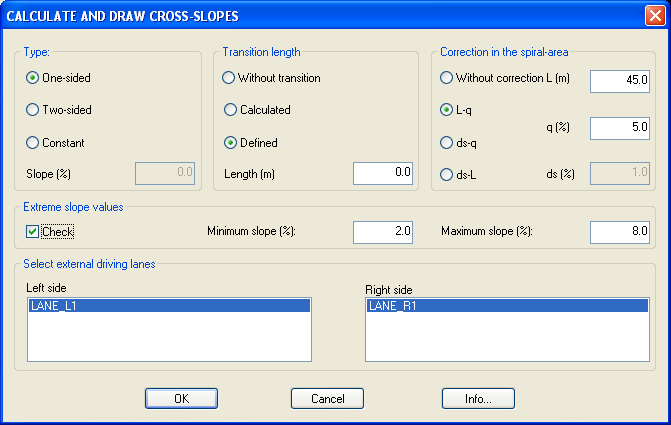
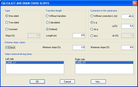
Parameters for cross slope calculation can be set by using the CALCULATE AND DRAW CROSS SLOPES dialog box:
There are several possibilities available when calculating cross slopes:
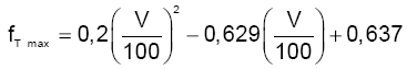
Inserting of one or two sided cross slope or constant slope[l16]
Inserting without transition, with calculated or defined transition;
In first case the cross slopes transition will be cascade.
In second case the transition length will be calculated according to the
following equation:
![]()
Where:
l transition length,
wid_l width of the left road line,
wid_d width of the right road line,
Vr calculation velocity.
In third case the length of the transition can be defined by user.
You can define transition-breaks by using one of the following methods:
without correction,
correction by parameters L and q,
correction by parameters
![]()
correction by parameters
![]()
Where parameters L, q and
![]()
L transition length,
q cross slope at the transition,
![]()
Parameter
![]()
![]()
Where:
q1 cross slope at the start of the transition,
q2 cross slope at the end of the transition,
wid1 width of the road at the start of the transition,
wid2 width of the road at the end of the transition and
L length of the transition.
After clicking OK, select left and right lane to be annotated.
 Several cross
slope lines get drawn to the cross slope rubric (even one above the other).
Cross slope lines get drawn on their layers. Layer names are:
LRO_WIDTH_lane-name_LEFT for lanes left to the axis and
LRO_WIDTH_lane-name_RIGHT for the lanes right to the axis.
Several cross
slope lines get drawn to the cross slope rubric (even one above the other).
Cross slope lines get drawn on their layers. Layer names are:
LRO_WIDTH_lane-name_LEFT for lanes left to the axis and
LRO_WIDTH_lane-name_RIGHT for the lanes right to the axis.
Program is calculating the cross slope based on starting and ending radius of the transition and radius of circular arc. At straight segments the cross slope is 2.5%. Cross slopes are calculated based on RADIUS/CROSS SLOPE for different calculating velocities.
Diagrams RADII/CROSS SLOPES are stored in file LRO_CrossFalls.xm and can be found in the directory where the PLATEIA is installed. According to the radius of circular arc or transition, cross slope Q is evaluated as follows:
If R < Rmin, then Q=7%;
If R is inside the interval covered by RADIUS/CROSS SLOPE diagram, Q is evaluated according to it;
If R > Rmax then Q=2.5%.
Program is calculating the cross slope based on starting and ending radius of the transition and radius of circular arc. At straight segments the cross slope is 2.5%. Cross slopes are calculated based on RADIUS/CROSS SLOPE (Figure 28, see Richtlinien fr die Anlage von Strasen, Teil Linienfhrung RAS-L, Ausgabe 1995, page 27) for different calculating velocities. RADII/CROSS SLOPES diagrams are stored in file LRO_CrossFalls.xm and can be found in the directory where the PLATEIA is installed. According to the radius of circular arc or transition, cross slope Q is evaluated as follows:
If R < Rmin, then Q=8%;
If R is inside the interval covered by RADIUS/CROSS SLOPE diagram, Q is evaluated according to it;
If R > Rmax ,then Q=2.5%.
Program is calculating the cross slope based on starting and ending radius of the transition and radius of circular arc. At straight segments the cross slope is 2.5%. Cross slopes are calculated based on RADIUS/CROSS SLOPE for different calculating velocities. The RADII/CROSS SLOPES diagrams are stored in file LRO_CrossFalls.xm and can be found in the directory where the PLATEIA is installed. According to the radius of circular arc or transition, cross slope Q is evaluated as follows:
If R < Rmin, then Q is evaluated based on calculation velocity according to the following table:
|
Vr |
|
|
|
|
|
|
|
|
|
|
|
Q |
|
|
|
|
|
|
|
|
|
|
If R is inside the interval covered by RADIUS/CROSS SLOPE diagram, Q is evaluated according to it;
If R > Rmax , then Q=2.5%.
Program is calculating the cross slope based on starting and ending radius of the transition and radius of circular arc. At straight segments the cross slope is 2.0%. The cross slopes are calculated according to the equation:
![]()
Where:
Vr calculating velocity v km/h,
R radius of circular arc or transition in m and
Q cross slope in %.
Program is calculating the cross slope based on starting and ending radius of the transition and radius of circular arc. At straight segments the cross slope is 2.0%. Cross slopes are calculated based on the RADIUS/CROSS SLOPE (Table 6.2, WZTZCZNE PROJEKTOWANIA DRG WPD-1, page 38 and Table 5.7, WZTZCZNE PROJEKTOWANIA DRG WPD-2, page 36) for different calculating velocities. The RADII/CROSS SLOPES diagrams are stored in file LRO_CrossFalls.xm and can be found in the directory where the PLATEIA 5.0 is installed. According to the radius of circular arc or transition, cross slope Q is evaluated as follows:
If R < Rmin, then Q=7%;
If R is inside the interval covered by RADIUS/CROSS SLOPE diagram, Q is evaluated according to it;
If R > Rmax , then Q=2.0%.
If the first element in an AXS file is straight segment, it is necessary to define the prefix of the transition or circular that follows.
Calculated cross slopes are drawn in the rubric Superelevations as two separate PLINE objects.
By setting the following parameters you can customize the appearance of superelevations:
[310601] Right superelevation-line-color (6),
[310602] Right superelevation-line-type (PL_HIDDEN),
[310603] Left superelevation-line-color (5),
[310604] Left superelevation-line-type (CONTINUOUS),
[310605] Superelevation scheme color (7).
Command name: Read cross-falls from file <- CRS
Command code: 31K2
Icon:
Task: Inserting the superelevations from a file
Input data: SUP file
Output data: Cross slope
Layers:
See also commands: 31K7
The Read cross-falls from file <- CRS (31K2) command inserts cross falls in the design based on data that was previously stored in a file of type CRS. File of this type can be created by using any ASCII text editor or by the Save cross-falls to file -> CRS (31K7) command.
See Appendix A for description of file structure.
Example of the CRS file:
# AXIS_0
KM M LANE_L2 LANE_L1 AXIS LANE_R1 LANE_R2 LANE_R3
0 0.0 00 2.50 2.50 -2.50 -2.50 -2.50
0 116.473 2.50 2.50 -2.50 -2.50 -2.50
0 209.103 7.0 0 7.0 0 -7.0 0 -7.0 0 -7.0 0
0 274.543 7.0 0 7.0 0 -7.0 0 -7.0 0 -7.0 0
The Read cross-falls from file <- CRS (31K2) command is mainly used in the following cases:
When the CRS file is created by entering the stations and the corresponding slope values through an ASCII text editor. Then cross slopes are automatically inserted in the drawing based on previously prepared CRS file.
When already created cross falls has to be corrected. In this case you first create the cross falls by using the CALCULATE AND DRAW CROSS-FALLS (31K1) command and then save the data to a SUP file type by using the Save cross-falls to file -> CRS (31K7) command. After correcting the slope values in the file that was previously saved by using ASCII text editor, you reinsert the cross falls in the design by using the Read cross-falls from file <- CRS (31K2) command.
Axis of superelevation is represented by a line along horizontal alignment and defines distance of rotation point from horizontal alignment. In most cases superelevation axis is defined on horizontal alignemnt. In special cases superelevation axes can be defined outside of horizontal alignemnt.
After we run the command we see next dialog box:
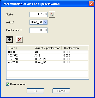
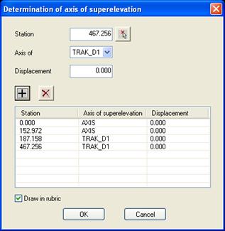
The Determination of axis of superelevation dialog box explanation:
|
Station |
User manually inserts station of superelevation axis change. With
button
|
|
Axis of |
User chooses axis of superelevation for selected station. User can choose between lanes that were set by command 21C3 or axis. |
|
Displacement |
Here user inserts displacement of axis of superelevation from selected lane in rubric Axis of superelevation. Positive values reprezent diplacement to the outside of axis, negative values to the inside. |
|
|
With this button we add new line of definition for axis of superelevation into list. With this button we also edit existing values. |
|
|
Deleting line from list. |
|
Draw in rubric |
On/off drawing the axis of superelevation in rubric. |
After we click OK we have set the axis of superelevation and programme will use it when saving in a LS file (command 31N). Values between stations are linear interpolated.
In case, that we don't set axis of superelevation, programme takes axis of superelevation by axis of road!
Command name:
Calculate cross-falls for
lanes
Command code: 31K3
Icon:

![]()
Task: selecting any cross slope for the
individual lanes
Input data: selected in a dialog box
Output data: cross falls
Layers:
See also commands: 31K1, 31K2
Using this command, you define cross falls for the individual lanes. You define slopes for an individual lane or for a lane group. You can even define slopes between any station and not only between the main elements.
Before invoking the 31K3 command, cross slope lines must be drawn in the cross slope rubric. You can use 31K1 or 31K2 commands.
After invoking the command, the following dialog box ppears:
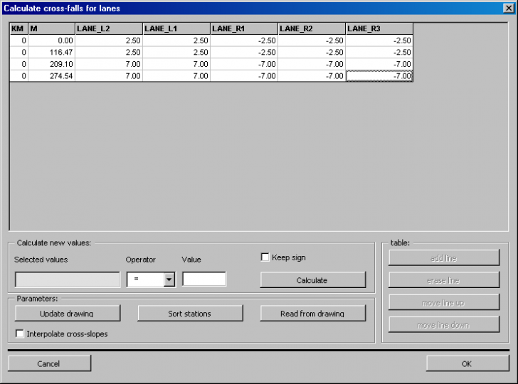
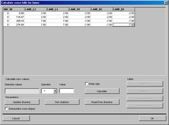
Cross slope definition procedure is as follows. First you select fields to which you want to change cross slopes in a table with written cross slopes. You can select either an individual field or field group (by dragging). By clicking the upper line containing the lane names, you select a complete column. Similarly, you can select all the lanes of a selected element by clicking the first column. Then you define cross slopes to the fields in the Calculate new values frame. You have three operators at your disposal:
= arranges a registered value for the selected fields,
+ adds a registered value for the selected fields,
- subtracts a registered value for the selected fields.
Using the Calculate button, selected values get calculated. By selecting keep sign option, selected fields keep their current sign. In addition, there are two more buttons:
Update in drawing draws values defined in a table to a cross slope rubric,
Sort stations if new lines were inserted you can sort them by stations,
Read from drawing reads values that are drawn in a cross slope rubric.
Command name:: Edit cross-falls in rubric
Command code: 31K3A
Icon: none
Task: editing cross-falls directly in rubric
Input data: cross-falls
Output data:
Layers:
See also commands: 31K1, 31K3, 31K3B
Command is used for editing cross-falls in rubric. With command 31K3A user edits cross-falls directly in rubric CROSS-FALLS. After invoking the command we must first select line of cross-fall that we want to edit. In drawing we see marked with yellow circle nearest vertex of line of cross-falls that was choosen.
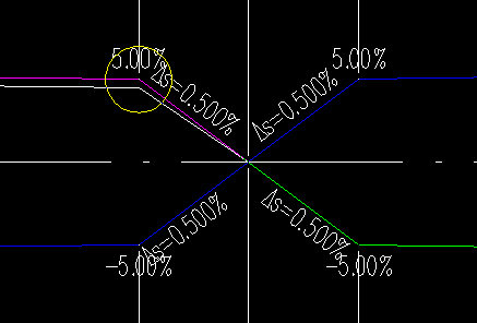
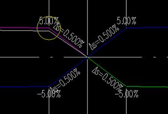
We get next dialog window:
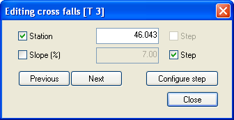
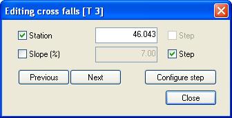
The Editing cross-falls dialog box explanation:
|
Station |
User can lock moving on choosen station and can regulate only slope. |
|
Slope |
User can lock slope and only change station of vertex. |
|
Previous |
Moving on previous vertex of line of cross-falls. |
|
Next |
Moving on next vertex of line of cross-falls. |
|
Configure step |
Opens dialog windov for configuring step |
User can with interactive input shange values of vertex of lines of cross-falls. To help user there is a dialog box, where there can be set step and can be locked change of stations or slopes.
Command name:: Edit cross-falls and lane elevations
Command code: 31K3B
Icon: none
Task: labeling
editing
cross-falls, lane elevations and jumps
Input data: cross-falls
and jumps
Output data:
Layers:
See also commands: command group
31K
Command is used for editing cross-falls for particular lanes. User has three options. First option is for editing values for cross-falls for particular lanes. In this case user enters value for cross-falls and programme automatically calculates lane elevations. Changes on neighbour lanes are calculate in way that function uses the same cross falls if it is possible.
Other two options are editing absolute and relative elevations. In both options user edits elevations on outside edges of lanes. When elevation is changed, user can see change on neighbourly lanes where slopes adjusted. All other slopes stay unchanged. Elevations cannot be edited in axis of superelevation, because elevations there are defined with elevation of vertical alignment.
Elevations and cross-falls are related to jumps between lanes. Jumps can be added, deleted and their properties can be changed along axis.
User can edit value in table, so that he chooses field in table and type in new value. In case, that user wants to change values in more fields, he must select more rows. If we press key SHIFT and select with mouse first and last row, there will be also selected all between the choosen rows. If we press CTRL key, we can choose more rows that are not neighbours. After we have selected rows, we select column, operand (+,- or =)and value. After we click Apply, values in table are recalculated.
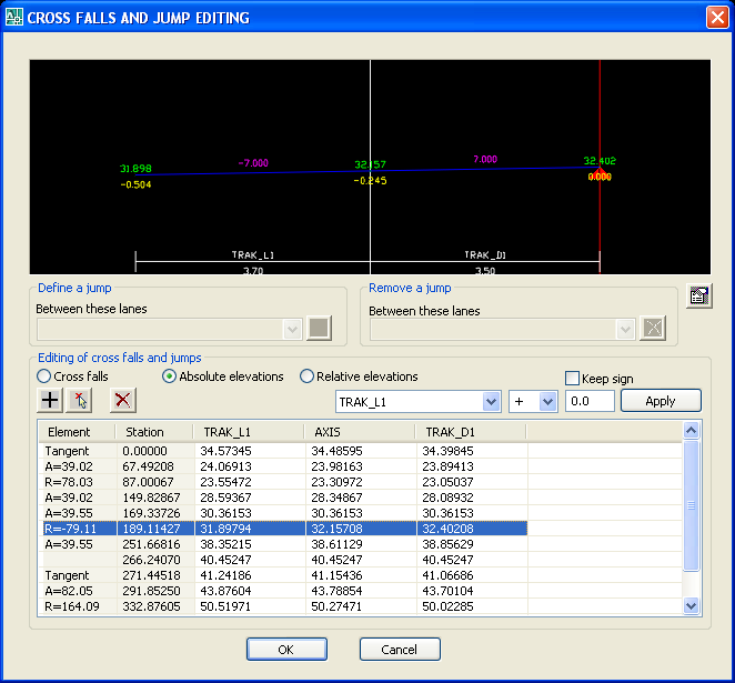
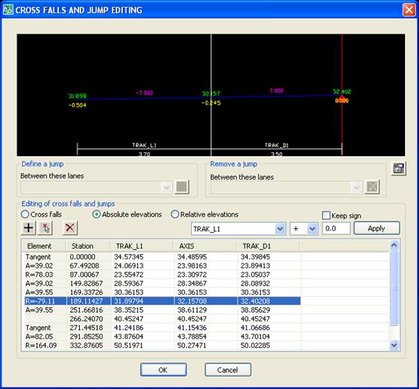
The Cross-falls and jump editing dialog box explanation:
|
Define a jump
|
Adding jump between choosen lanes. |
|
Remove a jump
|
Removing jump between choosen lanes. |
|
Cross falls |
Editing cross-falls elevations are calculated automatically. |
|
Absolute elevations |
Editing absolute elevations of outside edges of lanes cross-falls are calculated automatically. |
|
Relative elevations |
Editing relative elevations of outside edges of lanes cross-falls are calculated automatically. Elavations are relative to the axis of superelevation. |
|
Keep sign |
If we choose this option, user will increase/reduce absolute values of choosen fileds. |
|
Apply |
Calculation of choosen fields is carried out. Calculation is carried out based on operand, values and choosen column. |
|
|
Editing settings of cross-section view |
|
|
Adding line station into list. |
|
|
Adding line station with choosing station in drawing. |
|
|
Deleting choosen line. |
Triangle in cross-section view is marking axis of superelevation while circles are marking edges of lanes. Dialog window enables 'zoom' and 'pan' in so user can bring up that part of cross-fall, that is most interesting to him. When we press OK key, then values in the drawing are repared.
Command name: Read cross-falls from PLINE
Command code: 31K4
Icon:
Task: Converting PLINE object to superelevation
line
Input data:
Output data: Cross falls
Layers:
See also commands: 31O1
The Read cross-falls from PLINE (31K4) command is designed for a conversion of a PLINE object to a cross falls line. You have to decide if the converted PLINE object will become the left or the right cross slope. Then select the PLINE to be converted.
Command name: Calculate and label cross-falls
Command code: 31K5
Icon:

![]()
Task: Labeling of superelevations
Input data:
Output data:
Layers:
See also commands: 31K
The command is inserting the values of the cross slopes in the longitudinal section table together with the symbols that indicate the cross fall type - one or two sided. The slope differences (s) and distances where the difference appears are also marked.
Command name: Draw superelevation line
Command code: 31K6
Icon:
Task: Creating of the superelevation line based
on roadway widths and cross slopes
Input data: Roadway widths and cross slopes
Output data: Superelevation lines for right and left
side of the road
Layers: 31_SUPERELEV_LEFT_1, 31_SUPERELEV_RIGHT_1
See also commands: 31J1, 31K1
The Draw superelevaton line (31K6) command is inserting the superelevation lines for the left and right edge of the road in the rubric SUPERELEVATION. The superelevation is calculated for the start and endpoints of the main elements of horizontal alignment based on cross slopes and width of the roadway (together with expansions).
Command name: Save cross-falls to file -> CRS
Command code: 31K7
Icon:
Task: Writing of the superelevation data to a
file
Input data: Superelevation
Output data: SUP file
Layers:
See also commands: 31K2
You can save the data describing cross falls that was previously designed in the drawing. The command generates the CRS file type. The data should be saved when you need to redraw the cross falls later with or without changes that can be done by using any ASCII text editor.
See Appendix A for description of file structure.
Example of the CRS file:
# AXIS_0
KM M LANE_L2 LANE_L1 AXIS LANE_R1 LANE_R2 LANE_R3
0 0.0 00 2.50 2.50 -2.50 -2.50 -2.50
0 116.473 2.50 2.50 -2.50 -2.50 -2.50
0 209.103 7.0 0 7.0 0 -7.0 0 -7.0 0 -7.0 0
0 274.543 7.0 0 7.0 0 -7.0 0 -7.0 0 -7.0 0
Command is used to calculate cross-falls with median.
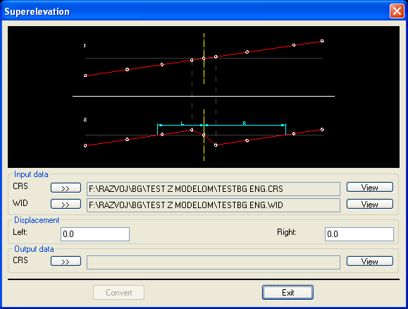
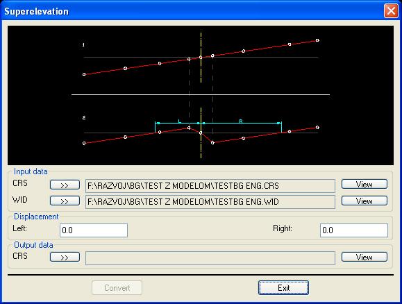
In dialog window user sets input data of cross-falls that were previously calculated and widths of the lanes. User defines points on left and right that will have the same elevation as it is defined for the vertical alignment. Before changing of super elevation the result is the same as it is seen in picture 1.
User defines output file. Result of transormation is shown on picture 2. Median lanes are adjusted in that way that points defined in Displacement frame have the same elevatioin as vertical alignment. Results are writen in new file and can be checked and edited with View button
Group code: 31L
Using the Vertical jumps between lanes command group, you define vertical jumps or curbs between lanes. Jump/curb data is saved by means of the 31N command to the LS file with which you insert a roadway to the longitudinal sections.
Command name: DEFINE VERTICAL JUMPS BETWEEN
LANES
Command code: 31L1
Icon:

![]()
Task: defining
of jumps for any lane and station
Input data:
Output data:
Layers: 31_JUMPS_RIGHT_name_lane,
31_JUMPS_LEFT_name_lane
See also commands: 31L, 31N
Using this command, you define jumps for individual lanes. You can define jumps for the individual lane or lane group. PLATEIA allows also defining of jumps between any station and not only between the main elements.
Jump is defined by the following two parameters:
delta h height difference between two neighboring lanes (vertical distance),
delta x spacing between two lanes (horizontal distance).
Parameter's meaning can be seen in the picture below.

Prior to invoking the 31L1 command, crossfall lines need to be previously drawn in the crossfall rubric.

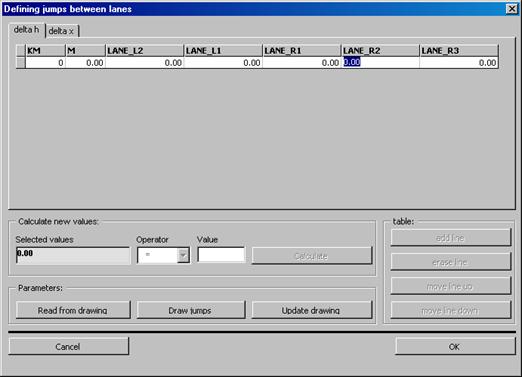
Jump definition procedure comprises a selection of fields in a table with written parameters. You define jumps by selecting an appropriate field using a mouse cursor, entering a value and confirming with ENTER. In addition, values can be calculated in the table.
Jump definition procedure
Select an individual field or field group (by dragging). By clicking the upper line (line with lane names), select a whole column. Similarly, select a whole line by clicking the first column (left to the KM column).
Define jumps in Calculate new values frame. There are three operators to choose from:
arranges entered values to the selected fields,
adds entered value to the selected fields,
- deducts entered value to the selected fields.
By clicking Calculate, selected values in table are calculated.
In addition, you can edit a table by means of the following commands:
Read from drawing reads values that are drawn in the jump rubrics,
Draw jumps draws values defined in the table in the jump rubric,
Update drawing change values defined in table in the jump rubric,
Add line adds a line to a table. You can select this command only when you have selected the whole line,
Erase line erases a line in a table. You can select this command only when you have selected the whole line,
Move line up/down moves a line in a table up/down. You can select this command only when you have selected the whole line.
Command name: READ JUMPS FROM FILE <-
JMP
Command code: 31L2
Icon:
Task: reading
of jumps from the JMP file
Input data: JMP
file
Output data: jumps
Layers: 31_JUMPS_RIGHT_name_lane,
31_JUMPS_LEFT_name_lane
See also commands: 31L
Using the Read jumps from file <- JMP (31L2) command, you insert jumps saved in the JMP file to the drawing. You can prepare the file manually or it can be a result of the Save jumps to file ->JMP (31L3) command.
You can find a structure of the JMP file in Appendix A.
Example of the JMP file:
KM M RADWEG SPURL2 SPURL1 OS SPURR1 SPURR2
0 0.0 0 0.20 0.05 0.0 0 0.0 0 0.0 0 0.0 0 0.0 0 0.0 0 0.0 0 0.0 0
0 20 0.0 0 0.20 0.05 0.0 0 0.0 0 0.0 0 0.0 0 0.0 0 0.0 0 0.0 0 0.0 0
0 50 0.0 0 0.20 0.05 0.0 0 0.0 0 0.0 0 0.0 0 0.0 0 0.0 0 0.0 0 0.0 0
0 80 0.0 0 0.20 0.05 0.0 0 0.0 0 0.0 0 0.0 0 0.0 0 0.0 0 0.0 0 0.0 0
0 938.77 0.20 0.05 0.0 0 0.0 0 0.0 0 0.0 0 0.0 0 0.0 0 0.0 0 0.0 0
Command name: SAVE JUMPS TO FILE->
JMP
Command code: 31L3
Icon:
Task: saving
of jumps to the JMP file
Input data: jumps
Output data: JMP
file
Layers: 31_JUMPS_RIGHT_name_lane,
31_JUMPS_LEFT_name_lane
See also commands: 31L
This command is intended for saving the jump values to the JMP file. You perform the save when you want to perserve jump data for some later inputting. You can find a structure of the JMP file in Appendix A.
Command Code: 31M
Command name: Label lanes and road edges
Command code: 31M
Icon:

![]()
Task: Drawing and labeling of road edges
Input data:
Output data: Road-edge lines
Layers:
See also commands:
This command calculates the elevation of the left and right road edge. Values of the calculated elevations are then written in the L.ROAD-EDGE ELEV and R.ROAD-EDGE ELEV rubrics of the longitudinal section table. If you want, program can also draw the curves of the left and right edge of the road.
Program calculates the elevation of every point of the alignment according to the following equation:
![]()
Where:
hig_l elevation of the left road edge [m],
hig_a elevation of the alignment [m],
q_l cross slope [%] and
wid_l width of the road (to the left of centerline).
Similar equation is used for calculation of the right road edge.
When you construct a highway with separated lines, there are two methods of calculation of the road edge elevations available. They are shown in the figure below:
In these two cases the width of the road is calculated according to the following equations:
1st Method
![]()
2nd Method
![]()
Where:
hig_l elevation of the left road edge [m],
hig_a elevation of the alignment [m],
q_l cross slope [%] and
wid_l width of the road (to the left of centerline).
Similar equation is used for calculation of the right road edge.
By setting the following parameters you can customize the appearance of road edges:
[310801] Roadway-edge elevation text-height (0.25),
[310802] Roadway-edge elevation text-alignment (_M),
[310803] Roadway-edge elevation text-color (7),
[310804] Right roadway-edge curve color (6),
[310805] Right roadway-edge curve linetype (LK_HIDDEN),
[310806] Left roadway-edge curve color (5),
[310807] Left roadway-edge curve linetype (CONTINUOUS).
Command Code: 31N
Command name: SAVE LONGITUDINAL SECTION -> LS
Command code: 31N
Icon:

![]()
Task: Writing the data defining longitudinal
section in a file
Input data:
Output data: LS file
Layers:
See also commands:
When the construction of the alignment is finalized, cross falls calculated, lane widths and jumps defined, you can store the data that defines the longitudinal section in a file of type LS. Data from this file is used for:
Calculate Volumes -> QV (31P1) command that calculates cut and fill volumes in the Longitudinal sections module,
Command from the Roadway (41F) group in the Cross sections module
Draw alignment and road edges in 3D <- LS command in the Axes module.
LS file type contains three data sections divided by the character &:
Data defining the curves in the alignment,
Data defining the minimums and maximums of the alignment,
Data defining stations, profile codes, alignment elevations, lanes cross falls, widths and jumps.
You can find a structure of the LS file in Appendix A.
EXTREM attribute can be evaluated as MIN for minimum or MAX for maximum of the alignment.
Example of the LS file:
# AXIS_0
CHAI VERT.ELEV R LON.SLO. SP EP
0.0 00 120.777 0.0 00 -4.160 0.0 00 0.0 00
154.961 114.331 1920 0.0 00 -3.398 81.806 228.116
301.558 109.350 750 0.0 00 -2.421 264.919 338.196
458.905 105.541 330 0.0 00 -1.177 438.373 479.436
50 0.0 00 105.057 0.0 00 0.0 00 50 0.0 00 50 0.0 00
&
*! STA ELEV EXTREME
120.777 MAX
105.057 MIN
&
LEFT SIDE RIGHT SIDE
*! CROSS_SECTION STATION ELEVATION ELEVATION ELEVATION ELEVATION ELEVATION ELEVATION ELEVATION
DISTANCE SLOPE DH SLOPE SLOPE SLOPE SLOPE
WIDTH DX WIDTH WIDTH WIDTH WIDTH
CROSS_SECTION STATION LANE_L2 JUMP_L1 LANE_L1 AXIS LANE_R1 LANE_R2 LANE_R3
P1 0.0 00 121.152 121.065 120.865 120.777 120.690 120.615 120.590
20.0 00 2.50 0 0.20 0 2.50 0 -2.50 0 -2.50 0 -2.50 0
7.0 00 0.050 3.50 0 3.50 0 6.50 0 7.50 0
P2 20.0 00 120.320 120.233 120.033 119.945 119.858 119.783 119.758
20.0 00 2.50 0 0.20 0 2.50 0 -2.50 0 -2.50 0 -2.50 0
7.0 00 0.050 3.50 0 3.50 0 6.50 0 7.50 0
P3 40.0 00 119.488 119.401 119.201 119.113 119.026 118.951 118.926
20.0 00 2.50 0 0.20 0 2.50 0 -2.50 0 -2.50 0 -2.50 0
7.0 00 0.050 3.50 0 3.50 0 6.50 0 7.50 0
P4 60.0 00 118.721 118.569 118.369 118.281 118.194 118.119 118.094
20.0 00 2.50 0 0.20 0 2.50 0 -2.50 0 -2.50 0 -2.50 0
9.591 0.050 3.50 0 3.50 0 6.50 0 7.50 0
P5 80.0 00 117.876 117.737 117.537 117.449 117.362 117.287 117.262
20.0 00 2.50 0 0.20 0 2.50 0 -2.50 0 -2.50 0 -2.50 0
9.054 0.050 3.50 0 3.50 0 6.50 0 7.50 0
P6 10 0.0 00 117.032 116.913 116.713 116.626 116.538 116.463 116.438
20.0 00 2.50 0 0.20 0 2.50 0 -2.50 0 -2.50 0 -2.50 0
8.238 0.050 3.50 0 3.50 0 6.50 0
Command Code: 31O
The group of commands named Rehabilitation enables you to efficiently design the reconstruction of the roadway. The Draw existing superelevations <- CRO (31O1) command is used to define the existing cross slopes along the roadway in order to design the new roadway that follows the old one as much as possible. The Calculate new vertical alignment -> TAN (31O2) command is used to calculate elevations of the alignment in the terrain profiles. For the definition of the elevation differences between the old and new road the Calculate thickness -> HD (31O3) command is available.
Command name: Draw existing superelevations <- CRO
Command code: 31O1
Icon:

![]()
Task: Defining the cross slope based on cross
section
Input data: CRO file
Output data: Line of the existing cross slope
Layers: 31_SUPERELEV_TMP
See also commands:
By using the Draw existing superelevations <- CRO (31O1) command, you can generate cross slopes of an existing road based on survey measurements of an existing road.
Survey data prepared as a file type CRO is the input needed for the calculation of cross slopes. The following figure shows an example of calculation of cross slope on one of the road profiles.
Figure: Calculation of cross slope.
Cross slope is calculated according to the following equation:
![]()
![]()
Where:
dx_l distance between centerline and left edge of the road [m],
dx_r distance between centerline and right edge of the road [m],
dy_l superelevation of the left edge of the road [m],
dy_r superelevation of the right edge of the road [m],
q_l left cross slope [%] in
q_r right cross slope [%].
If the calculated value of a cross slope exceeds 8%, the value is set to 8%.
Example of the CRO file:
# VERSION 1
P1 0+0.0 00
110.0 00 114.906
-11.0 00 112.754
-9.50 0 113.488
-8.80 0 113.676
-7.60 0 114.128
-6.20 0 114.324
-5.60 0 113.995
-4.50 0 114.374 ROADEDGE
-3.0 00 114.538
-2.0 00 114.642
-1.0 00 114.771
0.0 00 114.906 AXES
1.0 00 114.835
2.0 00 114.763
3.0 00 114.762
4.0 00 114.684
5.0 00 114.592
6.0 00 114.525 ROADEDGE
7.0 00 114.179
8.20 0 114.561
9.50 0 115.303
10.60 0 115.972
11.20 0 116.225
Program calculates the cross slopes for both left and right side of centerline based on three points:
Two points (left and right of centerline) with an ROADEDGE attribute and
One point on the road centerline.
For the profiles that do not have any point with the ROADEDGE attribute, program determines the leftmost point as a point on the left edge of the road and/or the rightmost point as a point on the right edge of the road.
If all the measured points belong to the
roadway only, the ROADEDGE attribute is not important. This attribute is
significant when there are also measured points outside of the roadway. In that
case, if the ROADEDGE attribute is missing, program will calculate an inaccurate
cross slope based on the leftmost and rightmost point of the profile.
Result of cross slope calculation are the lines drawn in the SUPERELEVATION rubric. Based on cross slopes of an existing road, you can design the superelevation of the new road.

By setting the following parameters you can customize the appearance of the design of superelevations of an existing road:
[310607] Existing right superelevation-curve color (241),
[310609] Existing right superelevation-curve linetype (LK_HIDDEN),
[310606] Existing left superelevation-curve color (141),
[310608] Existing left superelevation-curve linetype (CONTINUOUS).
Command name: Calculate new vertical alignment -> TAN
Command code: 31O2
Icon:

![]()
Task: Calculating new points of vertical
alignment when reconstructing the roadway
Input data: CRO file
Output data: TAN file and points on the alignment
Layers: 31_TANGENT_POINTS
See also commands:
After the cross slopes of an existing roadway have been calculated and the new ones designed, you have to define the elevation of the vertical alignment. Assuming the fact that you want to cover the roadway with an asphalt of appropriate minimal thickness, it is necessary to determine the point that will, with respect to the calculated cross slope, increase the vertical alignment to the highest possible level . See the figure that follows.
Elevation of the vertical alignment is calculated according to the following equation:
![]()
Where:
Q cross slope [%],
dist distance between the point and centerline [m],
dh thickness of the roadway coverage [m],
hig_p elevation of the point [m] in
hig_ali elevation of the new vertical alignment [m].
Example of the CRO file:
# VERSION 1
P1 0+0.0 00
110.0 00 114.906
-11.0 00 112.754
-9.50 0 113.488
-8.80 0 113.676
-7.60 0 114.128
-6.20 0 114.324
-5.60 0 113.995
-4.50 0 114.374 ROADEDGE
-3.0 00 114.538 ROADWAY
-2.0 00 114.642 ROADWAY
-1.0 00 114.771 ROADWAY
0.0 00 114.906 ROADWAY
1.0 00 114.835 ROADWAY
2.0 00 114.763 ROADWAY
3.0 00 114.762 ROADWAY
4.0 00 114.684 ROADWAY
5.0 00 114.592 ROADWAY
6.0 00 114.525 ROADEDGE
7.0 00 114.179
8.20 0 114.561
9.50 0 115.303
10.60 0 115.972
11.20 0 116.225
Program calculates the elevation of vertical alignment for every terrain point, separately for the left and right side of centerline, determines the highest point on the left and right side and at the end selects the highest of those two.
Similarly as with the Draw existing superelevations <- CRO (31O1) command, it is important which points are used for the calculation. As the reconstruction includes only roadway, program is filtering only points that have the ROADEDGE and ROADWAY attributes. If the Limit roadway-width box is not checked, the calculation will be applied to all the points independent of the attribute presence or its value.
If
the CRO file contains only points that belong to the roadway, the status of the
Limit roadway-width check box is not important. Its status is significant when
the file contains points outside of the roadway. In that case the box has to be
checked to filter only points which have the ROADEDGE and ROADWAY attributes.
In the Calculate new vertical alignment dialog box that appears after invoking the command, you have to select the input and output file names and if needed, select the Limit roadway-width check box and determine the minimum thickness.
Calculate new level dialog box.
Results of the calculation are the vertical alignment elevations in all the terrain profiles. These elevations are saved in a form of tangents. If the Draw levbel points box is checked, the calculated points will be inserted in the longitudinal section design on the 31_TANGENT_POINTS layer.
Layers:
See also commands 31O2
Program draws a new vertical alignment according to the tangent/vertical alignment calculation. Thus you can perform additional corrections and check the result again.
Command name: Result survey
Command code: 31O4
Icon:
Task: display
results
Input data: File
Output data: File
Layers:
See also commands: 31O2
The Result survey (31O4) command draws a final result of the new tangent position based on the tangent/vertical alignment calculation.
[l21] Command
name: Calculate thickness -> HD
Command code: 31O5
Icon:

![]()
Task: Labeling the elevation differences between
terrain and roadway
Input data: CRO file
Output data: HD file
Layers:
See also commands: 31O4
The Calculate thickness -> HD (31O3) command calculates the elevation differences between the terrain and roadway on the centerline and on both road edges. Program reads the terrain data form the CRO file type. The data that defines the roadway are taken from the longitudinal section design (alignment, superelevations, road widths). Calculated elevation differences are shown on the figure bellow:
Elevation differences are inserted in the appropriate rubric. The structure of the HD output file type is as follows:
PROF HD_L HD_AX HD_R
Codes description:
PROF profile code (STRING),
HD_L elevation difference on the left edge of the road in centimeters (REAL),
HD_AX elevation difference on the centerline in centimeters (REAL)
HD_R elevation difference on the right edge of the road in centimeters (REAL).

The HD File type can also contain lines that start with the following special characters:
Comment,
# SECTION start of a new section of data followed by the SECTION name,
Example of the HD file:
# VERSION 1
* PROF HD_L HD_AX HD_R
P1 14.906 10.351 6.028
P2 24.239 11.278 -8.655
P3 11.10 0 6.332 7.511
P4 18.647 2.263 3.0 00
P5 23.131 8.625 10.0 00
Command name: Save data for thickness-contours -> QS
Command code: 31O6
Icon:
Task: Saving of the elevation differences between
roadway and terrain
Input data: CRO file
Output data: QS file
Layers:
See also commands:
The Save data for thickness-contours -> QS (31O4) command is used to save the data defining the elevation differences between terrain and roadway on both left and right edge of the road and on its centerline. The command will save the data in a QS file type that can later be used by the program QuickSurf that will draw thickness contours in the DELTA H rubric.
The structure of the QS file type is the following:
X Y Z
Codes description:
X X coordinate of a rubric (REAL),
Y Y coordinate of a rubric (REAL)
Z Z coordinate (REAL).
QS file type example:
* X Y Z
9.850 6.435 14.906
9.850 5.997 10.351
9.850 5.778 6.028
10.706 6.435 24.239
10.706 5.997 11.278
10.706 5.778 -8.655
The QS file type does not support the sections of data.
Command Code: 31P
The Quick Volume-Calculation command group enables calculation of approximate cut and fill volumes according to the designed alignment. The idea is to optimize the distribution of cut and fill areas by changing the alignment of the designed object.
Command name: Calculate volumes -> QV
Command code: 31P1
Icon:
Task: Fast calculation of cut/fill volumes based
on the alignment and cross sections
Input data: LS and CRO files
Output data: QM file
See also commands: 31P2
This command is used to analyze the cut and fill areas on the designed section of the road. Program reads the necessary data from two files. First file, the LS file, contains the data that define vertical alignment elevation, road widths and cross slopes. Second file, the CRO file, contains the data describing the terrain from hatched cross sections. The resulting file is of type QM and contains cut and fills along the analyzed road section in individual profiles and as sum.
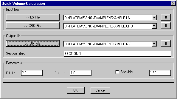

The Quick Volume-Calculation dialog box explanation:
|
LS file |
LS file name vertical alignment data, |
|
CRO file |
CRO file name cross section data, |
|
character # |
shows the available sections of data in a selected file, |
|
QM file |
output file name of type QS calculated results, |
|
Section label |
name of the section of data in the output file, |
|
Fill 1: |
approximate slope of fills, |
|
Cut 1: |
approximate slope of cuts, |
|
Shoulder |
approximate width of the shoulder, |
|
Excluded profiles |
list of cross sections excluded from the volume calculation (for example P1,P2, P3 or P1-P3). |
Structure of the LS and CRO type files is described in Appendix A. Result of the fast calculation of cut and fill volumes is saved in the QS file type that contains records of the following structure:
St. profile cut(m2) fill(m2) curr. cut(m3) curr. fill(m3)
-------- ----- ------ -------- ----- ------ --------
1 0.0 3.2
2 5.3 0.0 316.0 194.1
3 17.2 0.0 1214.4 194.1
4 5.0 36.6 2324.3 2024.6
5 0.1 19.6 2577.2 4833.4
6 0.0 26.0 2579.9 7113.7
7 0.0 32.9 2579.9 10 061.2
It is very important that the input files (LS and CRO) completely correspond. This means that every profile that appears in the LS file has to be defined in the CRO file. If an error is detected, the program will stop its execution.
Command name: Draw Volume-Line <- QV
Command code: 31P2
Icon:
Task: Drawing the volume line that represents cut
and fills along the road section
Input data: QV file
Output data: Volume line
See also commands: 31P1
The Draw Volume-Line <- QV (31P2) command is used to create a resulting volume line that represents exceeding cut and fill volumes in individual stations. It is inserted as the PLINE object on the 30_VOLUME_LINE layer. If the volume line is below the referential elevation, it is a cut volume, otherwise it is a fill volume.
Command Code: 31Q
Command name: Stop visibility length calculation
Command code: 31Q
Icon:

![]()
Task: Calculating and drawing of a stop sight
distance diagram
Input data: Velocity file (V) and level/longitudinal
slopes
Output data: Table
Function 31Q is used for analysis of vertical visibility and also for calculating stop visibility lengths. Stop visibility lengths are determined by design speed and longitudinal slope of vertical alignment.
Calculation of stop visibility lengths can be done in two ways. First one is with the following formula:

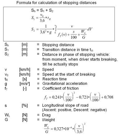
Second method is based on values that are stored in SHLIN.DAT file. The default values are set according to RAS-L standard. User can manually edit SHILIN.DAT file to customize table for local standard.
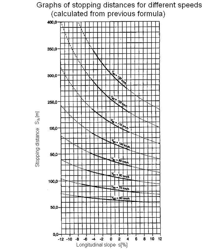
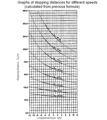
Values that are not defined in table are linearly interpolated. Results are represented in graph are two lines (for both driving directions). Lines are labeled with erf. Sh.
The other two lines represent vertical visibility in both driving directions. Lines are labeled with vorh. Sh. Vertical visibility is determined by the height of driver's eye and height ob obstacle on the roadway.
|
v85 [km/h] |
Height hZ [m] |
|
|
|
On sag curves there is also option to calculate night visibility. In that case lower of both values in applied on a graph. Rays of night visibility are represented with dashed lines. Night visibility is calculated regarding angle of light beam upward from the plane of the vehicle.
After you start the command following dialogue box appears.
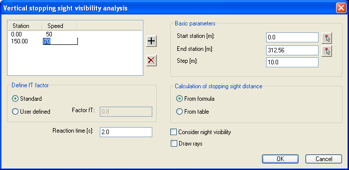
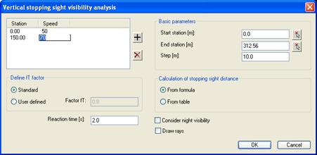
'Vertical stopping sight visibility analysis' dialog box explanation:
|
Station, Speed |
station and design speed of the section of the road |
|
|
adding new row (section) |
|
|
deleting row (section) |
|
Start stacionaa |
start station of vertical visibility analysis |
|
End stacionaa |
end station of vertical visibility analysis |
|
Step |
Step of calculation in meters |
|
Define
fT factor, |
friction
coefficient is calculated with following equation
|
|
Define
fT factor, |
user defines friction coefficient manually |
|
From formula |
Stopping sight distance is defined by upper formula |
|
From table |
Stopping sight distance is defined by SHLIN.DAT table |
|
Reaction time |
Reaction time of driver in seconds |
|
Consider night visibility |
If this option is on night visibility is checked also. |
|
Draw rays |
Rays of visibility are drawn in each step |
Command Code: 31R
Command name: Draw and save resultant slopeS -> RSL
Command code: 31R1
Icon:
Task: Schematic drawing of a resultant slope and
saving the data to a file
Input data:
Output data: RSL file
Layers:
See also commands: 31R2
The Draw and save resultant slope -> RSL (31R1) command is inserting the resultant slopes represented by arrows that show the direction of the slope. The length of the arrows indicates the value of the slope. Resultant slope is calculated and drawn for both left and right road edges.

Figure: Arrows showing the direction of the slope.
Resultant slopes can be saved in a RSL file that has the following record structure:
STA_KM STA_M RSL_L RSL_R
Codes description:
STA_KM station in kilometers (INTEGER),
STA_M station in meters (REAL),
RSL_L left resultant slope v % (REAL) in
RSL_R right resultant slope % (REAL).
Example of the RSL file:
* STA_KM STA_M RSL_L RSL_R
0 0.0 00 -4.92218 4.92218
0 20.0 00 -4.92218 4.92218
0 40.0 00 -4.92218 4.92218
0 60.0 00 -4.48139 4.48139
0 80.0 00 -3.83729 3.83729
0 10 0.0 00 -3.270 07 3.270 07
Command name: Save data for Roadway-Contours Calculation
-> QS
Command code: 31R2
Icon:
Task: Preparing the elevations of the roadway for
drawing of roadway contours
Input data:
Output data: QS file
Layers:
See also commands:
The Save data for Roadway-Contours Calculation -> QS (31R2) command extracts the elevations of the left and right roadway edge and the elevation of road centerline from the design. The data is then saved in the QS file type that can be used by the program QuickSurf which can later generate the roadway contours in the RESULTANT SLOPE rubric. In the dialog box that appears after invoking the command, you have to select the output file name and specify the distance between the profiles that will be saved.
The structure of the QS file type is as follows:
X Y Z
Description of the codes:
X X coordinate of a rubric (REAL),
Y Y coordinate of a rubric (REAL) in
Z Z coordinate (REAL).
Example of the QS file:
* X Y Z
9.850 6.435 14.906
9.850 5.997 10.351
9.850 5.778 6.028
10.706 6.435 24.239
10.706 5.997 11.278
10.706 5.778 -8.655
The QS file type does not support the sections of data.
Command name: Draw ditch
Command code: 31R3
Icon:

![]()
Task: Interactive drawing of vertical alignment
of ditches
Input data:
Output data:
Layers: 31_DITCH_LEFT, 31_DITCH_RIGHT
See also commands:
You can define the vertical alignment of ditches by simply selecting the points that will generate a PLINE object on the 31_DITCH_LEFT or 31_DITCH_RIGHT layers depending on the side of the road that you selected before. These objects can be edited by using the standard AutoCAD commands. When ready, you can label the vertical alignment of ditches by using the Calculate ditches (31R5) command. The longitudinal section design can contain any number of vertical alignments of ditches.
Command name: Read Ditch-Data from file <- DIT
Command code: 31R4
Icon:
Task: Batch input of the vertical alignment of
ditches
Input data: DIT file
Output data:
Layers: 31_DITCH_LEFT, 31_DITCH_RIGHT
See also commands:
The vertical alignment of ditches can also be inserted by using the Read Ditch-Data from file <- DIT (31R4) command that reads the selected DIT file. File of this type can be prepared by the appropriate command from the Cross sections module or by typing the data in any ASCII text editor.
The record structure of the DIT file is as follows:
STA_KM STA_M DIST HIG
Codes description:
STA_KM station in kilometers (INTEGER),
STA_Mstation in meters (REAL),
DISTdistance between ditch alignment and road centerline in meters (REAL),
HIG elevation of a ditch in meters (REAL).
Ditch alignment that is located left of the road centerline is represented by a negative distance value (DIST). Ditch alignment that is right of the road centerline is represented by a positive distance value (DIST).
The record in the DIT file type can start with following special characters:
Comment,
# SECTION Start of a new section of data followed by the SECTION name,
&Start of a new definition of ditch alignment.
The DIT file type example:
# DITCHES 5
STA_KM STA_M DIST HIG
0 0.0 00 4.5 114.92
0 20.0 00 4.5 114.57
0 40.0 00 4.5 114.33
0 60.0 00 4.5 114.07
0 80.0 00 4.5 113.83
0 10 0.0 00 4.5 113.27
&
0 85.0 00 -5.0 113.56
0 93.0 00 -5.0 114.57
0 120.0 00 -5.2 114.73
0 162.0 00 -5.2 115.79
0 186.0 00 -5.2 116.31
0 225.0 00 -5.2 116.14
Command name: Calculate ditches
Command code: 31R5
Icon:

![]()
Task: Labeling the ditches
Input data:
Output data:
Layers:
See also commands:
You can insert the labels defining the vertical alignment of ditches by using the Calculate ditches (31R5) command. The labels will be inserted in the L. DITCH ELEV. and R. DITCH ELEV rubrics depending on the side of the road where the ditch is located. Depending on the settings in the following dialog box, program will label the ditches in profiles and insert the labels that define ditch elevations and slopes.
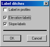
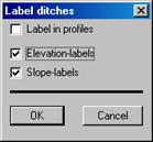
Command name: Save ditches to file -> DIT
Command code: 31R6
Icon: none
Task: Saving the data that define ditches in a
file
Input data:
Output data: DIT file
Layers:
See also commands:
The data that defines the vertical alignment of ditches can be saved in the DIT file type by using the Save ditches to file -> DIT (31R6) command. The vertical alignment of ditches can be reinserted in the drawing by invoking the Read Ditch-Data from file <- DIT (31R4) command. The structure of the DIT file type is described in a section that explains the Read Ditch-Data from file <- DIT (31R4) command. As distances between the road centerline and ditches are not defined in the Longitudinal sections module, the distances will be stored in the output file as 0.0 or 0.0 depending on the side of the road where the ditch is located.
Command code: 31S
Using this group of commands, you can insert sewer pipes and manholes to the longitudinal profiles. Pipe and manhole data can be annotated and saved to the files for later reading or manual processing. There is a preprepared table called PLATEIA SEWER SYSTEM containing all the needed rubrics for sewer data annotation.
This group of commands is specially usefull for users of Canalis. Sewer sistem can be designed with Canalis in same drawing as road axis. With command 21N4 in module Axis all necessary data is saved in .CAN file that can be inserted in longitudinal section.
Command name: Draw sewage system
Command code: 31S1
Icon:

![]()
Task: drawing of a sewer pipe
Input data:
Output data:
Layers: 31_PIPE, 31_PIPE_UPPER-EDGE
See also commands: 31S
You can insert a sewer pipe to the longitudinal profile by selecting intersection points with your mouse pointer. After invoking the command, insert a sewer pipe diameter in mm in a command line. Command line reads:
Pipe-diameter [mm] <10 00.0>:
You can insert points from the left side to the right side (in station direction). The line you are drawing shows a pipe bottom. You can insert intersection points simply by selecting them or you can help yourself by selecting parameters. If you type P in a command line, a dialog box opens in which you can define individual parameters or combine two of them.
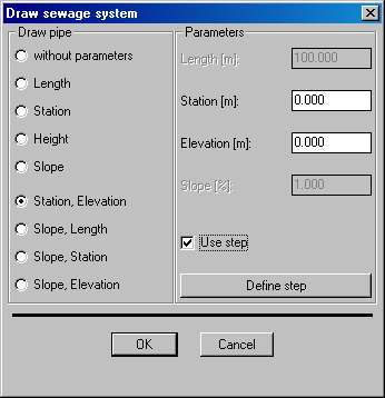
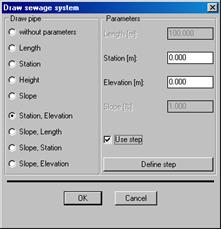
Command name: Label sewage system
Command code: 31S2
Icon:

![]()
Task: annotating of a sewer pipe
Input data: drawn pipe
Output data:
Layers:
See also commands: 31S
You can annotate sewer pipe data by using the 31S2 command to the rubric no. 27 called LEVEL LINE ELEV./FALL. Values get annotated between the sewer pipe intersections. Pipe bottom elevations in intersections and a pipe slope in between the neighboring intersections get inserted to the rubric.
Command name: Draw manholes in pipe vertices
Command code: 31S3
Icon:

![]()
Task: drawing of manholes in the sewer pipe
vertices
Input data:
Output data:
Layers: 31_MANHOLE
See also commands: 31S
This command enables drawing of manholes in the sewer pipe intersections. After invoking the command, the following dialog box appears:
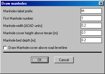
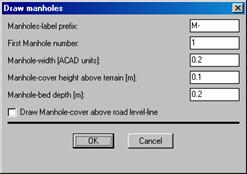
In the Insert manholes dialog box you can define parameters for labeling and drawing of manholes. If the Draw cover above vertical alignment option was selected, manhole gets drawn up to the vertical alignment. If not, manhole gets drawn up to a terrain line. Figure below shows an example of manhole drawn up to the terrain line.
You
will not get the Draw Manhole-cover
above road level-line command as an option, if you do not
have your vertical alignment drawn.
Command name: Label manholes
Command code: 31S4
Icon:

![]()
Task: labeling of sewer system manholes
Input data: from drawing
Output data:
Layers:
See also commands: 31S
You can label drawn manholes to the prepared rubrics by using the 31S3 command. This command annotates to the following three rubrics:
STATION/DISTANCE manhole station and distance between two neighboring manholes,
DISTANCE FROM AXIS horizontal distance of manhole from an axis (data can be in a form of a CAN file),
MANHOLE COVER ELEVATION manhole cover elevation.
Command name: Read pipe labels <- PIP
Command code: 31S5
Icon:
Task: inserting of pipe data from a PIP file
Input data: PIP file
Output data:
Layers:
See also command: 31S
This command enables insertion of data of pipe type to the PIPE DESCRIPTION rubric. Data should be prepared in a file of a PIP type. After invoking the command, you first select a PIP file you want to annotate and then a section from a list. After clicking OK, pipe type get annotated to the rubrics ordered stations.
You need to
prepare a file of PIP type in advance using any text editor such as Notepad
Structure and an example of PIP file are described in Appendix A.
Command name: Read sewage system <- SEW
Command code: 31S6
Icon:
Task: inserting of sewer from a CAN file
Input data: CAN file
Output data:
Layers: 31_PIPE, 31_PIPE_UPPER-EDGE, 31_MANHOLE
See also commands: 31S, 21N4
This command enables insertion of a road sewer system from a CAN file to a drawing. After invoking the command, the following dialog box appears:
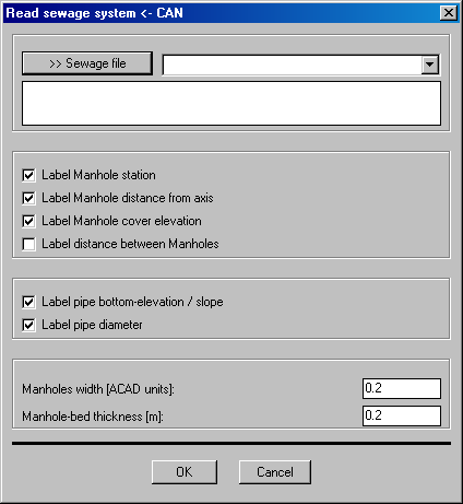

Using this dialog box, select a CAN file and a section. In addition, you can include a sewer rubric annotation. Using the lower frame of the dialog box, define manhole widths and manhole bed thicknesses as these are not defined in the CAN file.
You can save CAN file with command 21N4 in axes module.
You can see an example and a CAN file structure description in Appendix A.
Command name: Save sewage system -> CAN
Command code: 31S7
Icon:
Task: save sewage system to a CAN file
Input data: from drawing
Output data: CAN file
Layers: 31_PIPE, 31_PIPE_UPPER-EDGE, 31_MANHOLE
See also commands: 31S
Using this command, you save a sewer system from drawing to the CAN file.

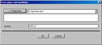
Using the Save sewer system dialog box, select a name and a CAN file path. If the file already exists, you can save its content to the existing section or type a new section name to a Section name field.
Sewer saved to the CAN file can be inserted by using the 31S6 command.
You can see an example and a description of CAN file structure in Appendix A.
Group code: 31U
The 31U command group is intended for preparation of longitudinal section for plotting. Using the 31U commands, you cut longitudinal section to the smaller sections and arrange them in a layout space. You plot the drawing by means of the layout space.
Command name: SET
BREAK AREA
Command code: 31U1
Icon:

![]()
Task: defining
of longitudinal section areas for breaking
Input data:
Plotting data:
Layers: 30_CONSTRUCTION_RECTANGLES
See also commands: 31U2, 31U3, 31U4
With command 31U1 the user breakes the longitudinal section into several plot frames in one of the three possible ways. Then the command 31U2 creates corresponding viewports in the paper space. After invoking the command, the following dialog box appears:
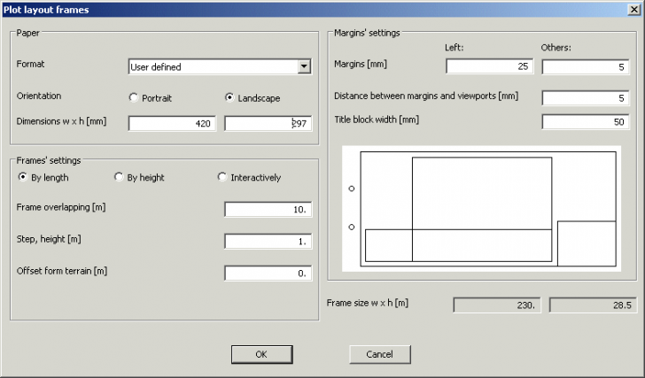
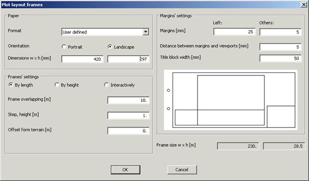
The Plot layout frames dialog box explanation:
|
Paper: Format,Orientation |
Select a proper paper format and choose orientation of frame (Landscape/Portrait). |
|
Paper: Dimension b x h (mm) |
Length and height of the paper in mm. If we choose one of preset paper format, the value is displayed automatically. |
|
Frames settings By length |
Break section according to the selected frame length (paper length minus edges). We can set overlapping of frames (by length), step for base elevation of the frame and the offset of the center of the frame from the terrain (by height). |
|
Frames settings By height |
Break section according to the selected frame height (paper format minus table height and edges). We can set overlapping of frames (by length step for base elevation of the frame and space above and below terrain in each frame. Length of frames can be shorter from the set value because of the restriction of the height. When calculating the frame length, the programme additionally checks for the space above and below terrain for all terrain points in one frame. |
|
Frames settings Interactively |
We can set step for height and length. When we click the OK button, the dialog box closes. We show the bottom left and upper right corners of the frames in the drawing. |
|
Margins' settings: Margins (mm) |
Define left and other margins on the paper |
|
Setting edges: Distance between margins and viewports (mm) |
Space between margin and viewport in paper space. |
|
Title block width (mm) |
Setting space on paper for title block. |
|
Frame size |
It shows the area in [m] that fits inside of one frame. |
Example Frames by length:
Example Frames by height:
Command name: ARRANGE
LONG. SECTION TO PLOT
Command code: 31U2
Icon:

![]()
Task: preparation
of longitudinal sections for plotting into layout space
Input data:
Plotting data:
Layers: 30_CONSTRUCTION_RECTANGLES
See also commands: 31U1
This command prepares longitudinal section for plotting. First select longitudinal section cutting areas. After invoking the command, program opens a new layout space and arranges profiles in it.
We can put frames of the longitudinal section in one or more layouts. When multiple layouts are selected, the programme makes a new layout for every frame. Name of layout space is composed of start and finish station. If we select single layout, the programme puts all frames in one layout. If we choose All frames into one table, all frames go into one table. In this case, the table heading is only displayed once.
If we want to use a title block, we can insert it into drawing by
checking the Title block option and
select it on the disk by clicking the button

![]() . If
we check the Fold to A4 option, the
programme will draw marks on the paper for folding to A4 format.[UB24]
. If
we check the Fold to A4 option, the
programme will draw marks on the paper for folding to A4 format.[UB24]
Command Code: 31V
Command name: Draw symbols <- SYM
Command code: 31V1
Icon:
Task: Inserting symbols that represent
intersections with utility infrastructure
Input data: SYM file
Output data:
Layers: 30_SYMBOLS
See also commands:
This command enables you to quickly insert the predefined blocks at the defined stations and elevations in the longitudinal section design. Data has to be prepared in the SYM file type that has the following record structure:
STA_KM STA_M HIGH BLOCK_NAME
Codes description:
STA_KM station in kilometers (INTEGER),
STA_M station in meters (REAL),
HIGH elevation in meters (REAL) in
BLOCK_NAME name of the block created by AutoCAD command BLOCK (STRING).
The file of type SYM can contain the records that start with following special characters:
# SECTION Start of a new section of data followed by the SECTION name,
Comment.
The SYM file type example:
STA_KM STA_M HIGH BLOCK_NAME
# Section1
0 0.0 00 114.92 PTT
0 25.780 114.57 CHANEL
0 83.056 113.83 CHANEL
0 284.450 113.27 PTT
The SYM file type can contain data sections.
Command name: Draw border-line <- IL
Command code: 31V2
Icon:
Task: Drawing lines along the axis in the
longitudinal section design
Input data: IL file
Output data: Border-line
Layers: 30_PLINES
See also commands: 31V3, 21M1, 21M4, 41K3, 41K4
By using the Draw border-line <- IL (31V2) command you can transfer the data that describe the lines along the axes, stored in the IL file type from the Axes or Cross sections modules in the design of longitudinal section. The IL file type can be generated by using the (2L6) command from the Axes module or by the (4I4) command from the Cross sections module.
Structure of the record in the IL file type is as follows:
KM M LINEi PROFIL LINEj
Codes description:
KM station in kilometers (INTEGER),
M station in meters (REAL),
LINEi desired
number of lines left of the axis (j=0, 1, 2 m),
where every line is defined by the pair:
Xi distance from the axis in meters (REAL),
Yi elevation in meters (REAL),
PROFIL profile code (STRING),
LINEj desired
number of lines right of the axis (j=0, 1, 2 m),
where every line is defined by the pair:
Xj distance from the axis in meters (REAL) and
Yj elevation in meters (REAL).
Records of the IL file type can contain the following special characters:
Comment,
# SECTION start of the new section of data followed by the SECTION name,
NULL replaces the value if it is not available for a certain station.
Example of the IL file type:
KM M FILL_L PROFIL CUT_R
0 -46.356 NULL NULL P1 NULL NULL
0 -34.919 NULL NULL P1A NULL NULL
0 -26.356 NULL NULL P2 NULL NULL
0 -6.356 NULL NULL P3 NULL NULL
0 13.644 NULL NULL P5 NULL NULL
0 21.076 NULL NULL P6 NULL NULL
0 33.644 NULL NULL P7 NULL NULL
0 53.644 NULL NULL P8 8.480 104.502
0 59.240 NULL NULL P9 12.427 104.210
0 73.644 NULL NULL P10 16.619 104.053
0 93.644 NULL NULL P11 15.464 103.734
0 112.967 NULL NULL P12 9.926 103.411
0 113.644 NULL NULL P13 9.616 102.442
0 123.018 NULL NULL P14 NULL NULL
0 133.644 11.789 110.30 0 P15 NULL NULL
0 153.644 15.851 114.320 P16 NULL NULL
0 166.695 13.071 115.560 P17 NULL NULL
0 173.644 10.911 120.073 P18 NULL NULL
0 177.968 9.293 124.308 P19 NULL NULL
In the Draw border-line dialog box below, you have to select the name of the input file of type IL, the desired section of data and the border-line that you want to insert in the longitudinal section design.

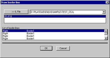
Program will insert a PLINE object that represents the selected border-line on the 30_PLINES layer.
Command name: Save border-line -> IL
Command code: 31V3
Icon:
Task: Drawing lines along the axis in the
longitudinal section
Input data: pline elements
Output data: IL file
Layers: 30_PLINES
See also commands: 31V2, 21M1, 21M4, 41K3, 41K4
This command enables saving a line along the axis. Saved lines can be inserted in cross-sections using the Layout data transfer<- IL (41K3) command. Data is transferred in the file of type IL.
You can see the description of CAN file structure in Appendix A.
KM M FILL_L PROFILE CUT_D
0 -46.356 NULL NULL P1 NULL NULL
0 -34.919 NULL NULL P1A NULL NULL
0 -26.356 NULL NULL P2 NULL NULL
0 -6.356 NULL NULL P3 NULL NULL
0 13.644 NULL NULL P5 NULL NULL
0 21.076 NULL NULL P6 NULL NULL
0 33.644 NULL NULL P7 NULL NULL
0 53.644 NULL NULL P8 8.480 104.502
0 59.240 NULL NULL P9 12.427 104.210
0 73.644 NULL NULL P10 16.619 104.053
0 93.644 NULL NULL P11 15.464 103.734
0 112.967 NULL NULL P12 9.926 103.411
0 113.644 NULL NULL P13 9.616 102.442
0 123.018 NULL NULL P14 NULL NULL
0 133.644 11.789 110.30 0 P15 NULL NULL
0 153.644 15.851 114.320 P16 NULL NULL
0 166.695 13.071 115.560 P17 NULL NULL
0 173.644 10.911 120.073 P18 NULL NULL
0 177.968 9.293 124.308 P19 NULL NULL
After invoking this command, the following dialog box appears:

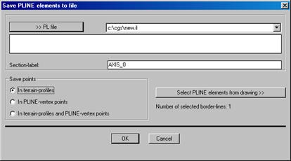
After pressing the>> IL file button, you show the way and name of the file you want to save. By using the Select PLINE elements from drawing >> button, you choose the lines you want to save to the IL file. Then you select a method of saving points.
You can save points:
in terrain profiles;
in vertices of the PLINE elements or
using both ways.
In addition, you can select also a file section. After clicking OK, the file is saved.
Command name: Auxiliary lines
Command code: 31V4
Icon:

![]()
Task: Drawing of a vertical, horizontal and
inclined auxiliary lines
Input data:
Output data: Construction lines
Layers: 30_CONSTR_LINES
See also commands:
By using the Auxiliary lines (31V4) command you can insert a vertical, horizontal and inclined auxiliary line. The vertical line will be inserted on the defined Station while Horizontal line will be inserted at specified elevation. In case of drawing inclined line user must define slope and insertion point of construction line.
The lines will be inserted on the 30_CONSTR_LINES layer.

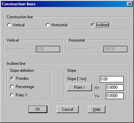
Command name: Define point, read station and elevation
Command code: 31V5
Icon:
Task: Measuring of a station and elevation of a
selected point
Input data:
Output data:
Layers:
See also commands:
The Define point, read station and elevation (31V5) command is similar to the AutoCAD ID command. The difference is that it takes into account the setting of horizontal and vertical scale of the current longitudinal section design. The command returns the station in kilometers and meters and elevation in meters.
Command name: Define station and elevation, draw point
Command code: 31V6
Icon:
Task: Drawing of a construction point
Input data:
Output data:
Layers: 30_CONSTR_LINES
See also commands:
The Define station and elevation, draw point (31V6) command inserts a construction point into the current longitudinal section design in a specified station at the given elevation. This command can become a useful tool when constructing the elements of the longitudinal section that are not drawn by the program automatically. Every construction point will be inserted on the 30_CONSTR_LINES layer.
Command name: LABEL POINT
Command code: 31V7
Icon:
Task: labeling
of values to a rubric in selected point
Input data: point
or station
Output data: value
in rubric
Layers:
See also commands: 31V9
Usually you label values to the rubrics in sections or points where values change (crossslopes). If you want to read and label a value in a point which is not necessarily a section, use the Label point command (31V7). After invoking the command, the Calculate in the selected point dialog box opens:

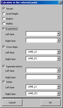
In the Calculate in the selected point dialog box, select rubrics and lanes to be labeled. After clicking OK, dialog box closes and the command line reads:
Point or station:
Select a labeling point using a mouse or insert its station in m. Finish labeling by clicking Enter.
Command name: Dimension elevations
Command code: 31V81
Icon:

![]()
Task: Dimensioning of an elevation
Input data:
Output data:
Layers: 30_CONSTR_LINES
See also commands:
The elevation of any desired longitudinal section element could be dimensioned by using the Dimension elevations (31V81) command. Using the Dimension elevations dialog box shown below that appears after invoking the command, you can define the dimensioning style. The dimension of the defined style will then be inserted at the selected point together with its elevation label.
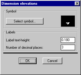
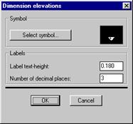
Command name: Dimension slope
Command code: 31V82
Icon:

![]()
Task: Dimensioning of a slope
Input data:
Output data:
Layers: 30_CONSTR_LINES
See also commands:
By using the Dimension slope (31V82) command you can draw a dimension of any desired slope in the current longitudinal section design. Through the Dimension slope dialog box shown below that appears after invoking the command you can define the dimensioning style (type of arrow and slope label). At the end you have to select two points that define the position of the slope dimension.
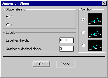
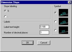
Command name: DIMENSION LENGTH
Command code: 31V8
Icon:
Task: dimensioning
of LINE element or dimensioning between two points
Input data: from
drawing
Output data: modified
drawing
Layers: this
command does not use them
See also commands: 31V8
Using the 31V83 command, you can dimension longitudinal section elements. This command takes into account both horizontal and vertical scale and so differs from the usual dimensioning using the AutoCAD commands. You can perform dimensioning between two selected points or select LINE elements.
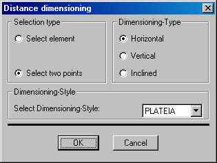
You can dimension horizontal, vertical or inclined distance between two selected points. In the Dimensioning style frame select a dimensioning stile from the styles defined in AutoCAD.
Command name: LABEL PLINE
Command code: 31V9
Icon:
Task: annotating
of polyline to user rubric
Input data: polyline
in drawing
Output data: data
in rubric
Layers:
See also commands: 31V7, 31C3
This command is intended for annotating of polyline to user rubric. You can annotate a station, elevation, height-difference between the selected polyline and tarrain or a height-difference between a selected polyline and any polyline.
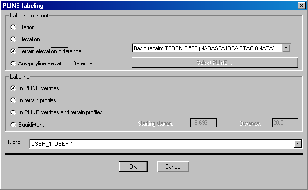

Select between annotating in polyline vertex points, in cross-section points or on selected even distance.
Prior to invoking the command, you need to have prepared a user rubric first. You can add it using the 31C3 command.
Command name: Insert text from file <- TXT
Command code: 31VA
Icon:
Task: Reading text from file at specified station
and elevation
Input data: TXT file
Output data:
Layers:
See also commands: 31VB
This command enables a quick insertion of any text on previously selected stations and elevations in a longitudinal section. The command takes into account text parameters such as elevation, rotation, leveling, style and layer. You prepare data in a TXT file having the following form:
STA_KM STA_M ELEV TEXT TXT_HEIGHT TXT_ROT TXT_LEVEL TXT_FONT LAYER COLOR
Legend:
STA_KM station in km (INTEGER),
STA_M station in m (REAL),
ELEV elevation in m (REAL),
TEXT text content that needs to be in inverted commas (STRING),
TXT_HEIGHT text height (REAL),
TXT_ROT text rotation (REAL),
TXT_LEVEL text leveling (STRING),
TXT_STYLE text style that needs to appear in inverted commas () and
LAYER text layer (STRING)
COLOR text color that needs to appear in inverted commas ().
In HD file, also the lines having a special symbol in the first column may appear. Special symbols are as follows:
asterix in first column stands for comment or comment line,
Example of TXT file:
* STA_KM STA_M ELEV TEXT TXT_HEIGHT TXT_ROT TXT_LEVEL TXT_STYLE LAYER
10,0 00 115,0 00 'KRIANJE' 0,350 0,0 00 BL 'TXT' 'TEKSTI 1'
40,0 00 114,0 00 'DALJNOVOD' 0,250 0,0 00 TR 'RUBRIC_TXT' 'TEKSTI 2'
120,0 00 102,0 00 'PREHOD 2' 0,40 0 90,0 00 R
130,0 00 104,0 00 'PREHOD 3' 0,30 0 0,0 00
140,0 00 106,0 00 'PREHOD 4'
150,0 00 107,0 00 'PREHOD 5' 0,10 0 NULL NULL 'TXT' 'TEKSTI 3'
First four columns in TXT file are obligatory while the rest of them are not. You must replace the missing intermediate values with the NULL symbol. See Example of TXT file.

TXT file has no sections.
Command name: Save text to file -> TXT
Command code: 31VB
Icon:
Task: Saving any text at specified station and
elevation to file
Input data: Selected texts in drawing
Output data: TXT file
Layers:
See also commands: 31VA
This command enables saving of any text in longitudinal section to the TXT file that you can read again by using the Read text from file <-TXT (31VA) command. Saved file has a structure as described with the Read text from file <-TXT (31VA) command. First you specify the name of TXT file to which you will save your data and then you select TEXT elements to be saved.
TXT file has no sections.
[UB1]Changed in 20 07. Command group I doesn't exist any more
[l2]Novost P20 06
[l3]P20 06
[l4]Novost prevod P20 06
[l5]Prevod P20 06
[l6]Prevod P20 06
[l7]Prevod P20 06
[l8]Prevod P20 06
[l9]Prevod P20 06
[l10]P20 06
[l11]Prevod P20 06
[l12]Novo P20 06
[l13]Nov sklop, prevod P20 06
[UB14]Novo v 20 08
[l15]posodobljeno
[l16]posodobljeno
[UB17]Novo v 20 08
[UB18]Novo v 20 07-prevod 20 08
[UB19]Updated in 20 08
[l20]posodobljneo P20 06
[l21]P20 06
|
Politica de confidentialitate | Termeni si conditii de utilizare |

Vizualizari: 2119
Importanta: ![]()
Termeni si conditii de utilizare | Contact
© SCRIGROUP 2024 . All rights reserved