COMPUTATIONAL GEOMETRY

Computational geometry is the branch of computer science that studies algorithms for solving geometric problems. In modern engineering and mathematics, computational geometry has applications in, among other fields, computer graphics, robotics, VLSI design, computer-aided design, and statistics. The input to a computational-geometry problem is typically a description of a set of geometric objects, such as a set of points, a set of line segments, or the vertices of a polygon in counterclockwise order. The output is often a response to a query about the objects, such as whether any of the lines intersect, or perhaps a new geometric object, such as the convex hull (smallest enclosing convex polygon) of the set of points.

In this chapter, we look at a few computational-geometry algorithms in two dimensions, that is, in the plane. Each input object is represented as a set of points , where each p_i = (x_i, y_i) and x_i, y_i R. For example, an n-vertex polygon P is represented by a sequence p₀, p₁, p₂, . . . , p_n-1 of its vertices in order of their appearance on the boundary of P. Computational geometry can also be performed in three dimensions, and even in higher- dimensional spaces, but such problems and their solutions can be very difficult to visualize. Even in two dimensions, however, we can see a good sample of computational-geometry techniques.

Section 1 shows how to answer simple questions about line segments efficiently and accurately: whether one segment is clockwise or counterclockwise from another that shares an endpoint, which way we turn when traversing two adjoining line segments, and whether two line segments intersect. Section 2 presents a technique called 'sweeping' that we use to develop an O(n lg n)-time algorithm for determining whether there are any intersections among a set of n line segments. Section 3 gives two 'rotational-sweep' algorithms that compute the convex hull (smallest enclosing convex polygon) of a set of n points: Graham's scan, which runs in time O(n 1g n), and Jarvis's march, which takes O(nh) time, where h is the number of vertices of the convex hull. Finally, Section 4 gives an O(n 1g n)-time divide-and-conquer algorithm for finding the closest pair of points in a set of n points in the plane.

1 Line-segment properties

Several of the computational-geometry algorithms in this chapter will require answers to questions about the properties of line segments. A convex combination of two distinct points p₁ = (x₁, y₁) and p₂ = (x₂, y₂) is any point p₃ = (x₃, y₃) such that for some in the range 0 1, we have x₃ = ax₁ + (1 - )x₂ and y₃ = y₁ + (1 - )y_2. We also write that p₃ = p₁ + (1 - )p_2. Intuitively, p₃ is any point that is on the line passing through p₁ and p₂ and is on or between p₁ and p₂ on the line. Given two distinct points p₁ and p2, the line segment is the set of convex combinations of p₁ and p₂. We call p₁ and p₂ the endpoints of segment . Sometimes the ordering of p₁ and p₂ matters, and we speak of the directed segment . If p₁ is the origin (0, 0), then we can treat the directed segment as the vector p₂.

In this section, we shall explore the following questions:

There are no restrictions on the given points.

We can answer each question in O(1) time, which should come as no surprise since the input size of each question is O(1). Moreover, our methods will use only additions, subtractions, multiplications, and comparisons. We need neither division nor trigonometric functions, both of which can be computationally expensive and prone to problems with round-off error. For example, the 'straightforward' method of determining whether two segments intersect--compute the line equation of the form y = mx + b for each segment (m is the slope and b is the y-intercept), find the point of intersection of the lines, and check whether this point is on both segments uses division to find the point of intersection. When the segments are nearly parallel, this method is very sensitive to the precision of the division operation on real computers. The method in this section, which avoids division, is much more accurate.

Cross products

Computing cross products is at the heart of our line-segment methods. Consider vectors p₁ and p₂, shown in Figure 1(a). The cross product p₁ x p₂ can be interpreted as the signed area of the parallelogram formed by the points (0, 0), p₁, p₂, and p₁ + p₂ = (x₁ + x₂, y₁ + y₂₎. An equivalent, but more useful, definition gives the cross product as the determinant of

Figure 1 (a) The cross product of vectors p₁ and p₂ is the signed area of the parallelogram. (b) The lightly shaded region contains vectors that are clockwise from p. The darkly shaded region contains vectors that are counterclockwise from p.

a matrix:¹

^{1 Actually, the cross product is a three-dimensional concept. It is a vector that is perpendicular to both p and p according to the 'right-hand rule' and whose magnitude is |x y - x y |. In this chapter, however, it will prove convenient to treat the cross product simply as the value x y - x y}

^{If p X p is positive, then p is clockwise from p with respect to the origin (0, 0); if this cross product is negative, then p is counterclockwise from p . Figure 1(b) shows the clockwise and counterclockwise regions relative to a vector p. A boundary condition arises if the cross product is zero; in this case, the vectors are collinear, pointing in either the same or opposite directions.}

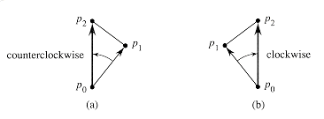
^{To determine whether a directed segment is clockwise from a directed segment with respect to their common endpoint p , we simply translate to use p as the origin. That is, we let p - p denote the vector p' = (x , y' where x' = x - x and y' = y - y , and we define p - p similarly. We then compute the cross product}

^{(p - p ) x (p - p ) = (x - x ) (y - y ) - (x - x ) (y - y}

If this cross product is positive, then is clockwise from ; if negative, it is counterclockwise.

Determining whether consecutive segments turn left or right

Our next question is whether two consecutive line segments turn left or right at point p_l. Equivalently, we want a method to determine which way a given angle p₀p₁p₂ turns. Cross products allow us to answer this question without computing the angle. As shown in Figure 2, we simply check whether directed segment is clockwise or counterclockwise relative to directed segment . To do this, we compute the cross product (p₂ - p₀) X (p₁ - p₀). If the sign of this cross product is negative, then is counterclockwise with respect to , and thus we make a left turn at P₁. A positive cross product indicates a clockwise orientation and a right turn. A cross product of 0 means that points p₀, p₁, and p₂ are collinear.

Figure 2 Using the cross product to determine how consecutive line segments turn at point p₁. We check whether the directed segment is clockwise or counterclockwise relative to the directed segment . (a) If counterclockwise, the points make a left turn. (b) If clockwise, they make a right turn.

Determining whether two line segments intersect

We use a two-stage process to determine whether two line segments intersect. The first stage is quick rejection: the line segments cannot intersect if their bounding boxes do not intersect. The bounding box of a geometric figure is the smallest rectangle that contains the figure and whose segments are parallel to the x-axis and y-axis. The bounding box of line segment is represented by the rectangle with lower left point and upper right point , where . Two rectangles, represented by lower left and upper right points , intersect if and only if the conjunction

is true. The rectangles must intersect in both dimensions. The first two comparisons above determine whether the rectangles intersect in x; the second two comparisons determine whether the rectangles intersect in y.

The second stage in determining whether two line segments intersect decides whether each segment 'straddles' the line containing the other. A segment straddles a line if point p₁ lies on one side of the line and point p₂ lies on the other side. If p₁ or p₂ lies on the line, then we say that the segment straddles the line. Two line segments intersect if and only if they pass the quick rejection test and each segment straddles the line containing the other.

Figure 3 Determining whether line segment straddles the line containing segment . (a) If it does straddle, then the signs of the cross products (p₃ - p₁) x (p₂ - p₁) and (p₄ - p₁) x (p₂ - p₁) differ. (b) If it does not straddle, then the signs of the cross products are the same. (c)-(d) Boundary cases in which at least one of the cross products is zero and the segment straddles. (e) A boundary case in which the segments are collinear but do not intersect. Both cross products are zero, but they would not be computed by our algorithm because the segments fail the quick rejection test--their bounding boxes do not intersect.

We can use the cross-product method to determine whether line segment straddles the line containing points p₁ and p₂. The idea, as shown in Figures 3(a) and (b), is to determine whether directed segments and have opposite orientations relative to . If so, then the segment straddles the line. Recalling that we can determine relative orientations with cross products, we just check whether the signs of the cross products (p₃ - p₁) X (p₂ - p₁) and (p₄ - p₁) X (p₂ - p₁) are different. A boundary condition occurs if either cross product is zero. In this case, either p₃ or p₄ lies on the line containing segment . Because the two segments have already passed the quick rejection test, one of the points p₃ and p₄ must in fact lie on segment . Two such situations are shown in Figures 3(c) and (d). The case in which the two segments are collinear but do not intersect, shown in Figure 3(e), is eliminated by the quick rejection test. A final boundary condition occurs if one or both of the segments has zero length, that is, if its endpoints are coincident. If both segments have zero length, then the quick rejection test suffices. If just one segment, say , has zero length, then the segments intersect if and only if the cross product (p₃ - p₁) x (p₂ - p₁) is zero.

Other applications of cross products

Later sections of this chapter will introduce additional uses for cross products. In Section 3, we shall need to sort a set of points according to their polar angles with respect to a given origin. As Exercise 1-2 asks you to show, cross products can be used to perform the comparisons in the sorting procedure. In Section 2, we shall use red-black trees to maintain the vertical ordering of a set of nonintersecting line segments. Rather than keeping explicit key values, we shall replace each key comparison in the red-black tree code by a cross-product calculation to determine which of two segments that intersect a given vertical line is above the other.

Exercises

Prove that if p₁ X p₂ is positive, then vector p₁ is clockwise from vector p₂ with respect to the origin (0, 0) and that if this cross product is negative, then p₁ is counterclockwise from p₂.

Write pseudocode to sort a sequence p , p , . . . . ,p_n) of n points according to their polar angles with respect to a given origin point p . Your procedure should take 0(n lg n) time and use cross products to compare angles.

Show how to determine in 0(n² 1g n) time whether any three points in a set of n points are collinear.

Professor Amundsen proposes the following method to determine whether a sequence p₀, p , p_n-1 of n points forms the consecutive vertices of a convex polygon. (See Section 16.4 for definitions pertaining to polygons.) Output 'yes' if the set , where subscript addition is performed modulo n, does not contain both left turns and right turns; otherwise, output 'no.' Show that although this method runs in linear time, it does not always produce the correct answer. Modify the professor's method so that it always produces the correct answer in linear time.

Given a point p₀ = (x₀, y₀), the right horizontal ray from p₀ is the set of points , that is, it is the set of points due right of p₀ along with p₀ itself. Show how to determine whether a given right horizontal ray from p₀ intersects a line segment in O(1) time by reducing the problem to that of determining whether two line segments intersect.

One way to determine whether a point p₀ is in the interior of a simple, but not necessarily convex, polygon P is to look at any ray from p₀ and check that the ray intersects the boundary of P an odd number of times but that p₀ itself is not on the boundary of P. Show how to compute in (n) time whether a point p₀ is in the interior of an n-vertex polygon P. (Hint: Use Exercise 1-5. Make sure your algorithm is correct when the ray intersects the polygon boundary at a vertex and when the ray overlaps a side of the polygon.)

Show how to compute the area of an n-vertex simple, but not necessarily convex, polygon in (n) time.

2 Determining whether any pair of segments intersects

This section presents an algorithm for determining whether any two line segments in a set of segments intersect. The algorithm uses a technique known as 'sweeping,' which is common to many computational-geometry algorithms. Moreover, as the exercises at the end of this section show, this algorithm, or simple variations of it, can be used to solve other computational-geometry problems.

The algorithm runs in O(n lg n) time, where n is the number of segments we are given. It determines only whether or not any intersection exists; it does not print all the intersections. (By Exercise 2-1, it takes (n ) time in the worst case to find all the intersections in a set of n line segments.)

In sweeping, an imaginary vertical sweep line passes through the given set of geometric objects, usually from left to right. The spatial dimension that the sweep line moves across, in this case the x-dimension, is treated as a dimension of time. Sweeping provides a method for ordering geometric objects, usually by placing them into a dynamic data structure, and for taking advantage of relationships among them. The line-segment-intersection algorithm in this section considers all the line-segment endpoints in left-to-right order and checks for an intersection each time it encounters an endpoint.

Our algorithm for determining whether any two of n line segments intersect makes two simplifying assumptions. First, we assume that no input segment is vertical. Second, we assume that no three input segments intersect at a single point. (Exercise 2-8 asks you to describe an implementation that works even if these assumptions fail to hold.) Indeed, removing such simplifying assumptions and dealing with boundary conditions is often the most difficult part of programming computational-geometry algorithms and proving their correctness.

Figure 4 The ordering among line segments at various vertical sweep lines. (a) We have a >_r c, a >_t b, b >_t c, a >_t c, and b >_u c. Segment d is comparable with no other segment shown. (b) When segments e and f intersect, their orders are reversed: we have e >_v f but f >_w e. Any sweep line (such as z) that passes through the shaded region has e and f consecutive in its total order.

Ordering segments

Since we assume that there are no vertical segments, any input segment that intersects a given vertical sweep line intersects it at a single point. We can thus order the segments that intersect a vertical sweep line according to the y-coordinates of the points of intersection.

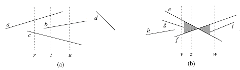
To be more precise, consider two nonintersecting segments s and s We say that these segments are comparable at x if the vertical sweep line with x-coordinate x intersects both of them. We say that s_l is above s₂ at x, written s₁ > X s₂, if s and s are comparable at x and the intersection of s with the sweep line at x is higher than the intersection of s with the same sweep line. In Figure 4(a), for example, we have the relationships a >_r c, a >_t b, b >_t c, a >_t c, and b >_u c. Segment d is not comparable with any other segment.

For any given x, the relation '>_x' is a total order (see Section 5.2) on segments that intersect the sweep line at X_. The order may differ for differing values of x_, however, as segments enter and leave the ordering. A segment enters the ordering when its left endpoint is encountered by the sweep, and it leaves the ordering when its right endpoint is encountered.

What happens when the sweep line passes through the intersection of two segments? As Figure 4(b) shows, their positions in the total order are reversed. Sweep lines v and w are to the left and right, respectively, of the point of intersection of segments e and f, and we have e >_v f and f >_w e. Note that because we assume that no three segments intersect at the same point, there must be some vertical sweep line x for which intersecting segments e and f are consecutive in the total order >_x. Any sweep line that passes through the shaded region of Figure 4(b), such as z, has e and f consecutive in its total order.

Moving the sweep line

Sweeping algorithms typically manage two sets of data:

1. The sweep-line status gives the relationships among the objects intersected by the sweep line.

2. The event-point schedule is a sequence of x-coordinates, ordered from left to right, that defines the halting positions of the sweep line. We call each such halting position an event point. Changes to the sweep-line status occur only at event points.

For some algorithms (the algorithm asked for in Exercise 2-7, for example), the event-point schedule is determined dynamically as the algorithm progresses. The algorithm at hand, however, determines the event points statically, based solely on simple properties of the input data. In particular, each segment endpoint is an event point. We sort the segment endpoints by increasing x-coordinate and proceed from left to right. We insert a segment into the sweep-line status when its left endpoint is encountered, and we delete it from the sweep-line status when its right endpoint is encountered. Whenever two segments first become consecutive in the total order, we check whether they intersect.

The sweep-line status is a total order T, for which we require the following operations:

INSERT(T, s): insert segment s into T.

DELETE(T, s): delete segment s from T.

ABOVE(T, s): return the segment immediately above segment s in T.

BELOW(T, s): return the segment immediately below segment s in T.

If there are n segments in the input, we can perform each of the above operations in O(lg n) time using red-black trees. Recall that the red-black-tree operations in Chapter 14 involve comparing keys. We can replace the key comparisons by cross-product comparisons that determine the relative ordering of two segments (see Exercise 2-2).

Segment-intersection pseudocode

The following algorithm takes as input a set S of n line segments, returning the boolean value TRUE if any pair of segments in S intersects, and FALSE otherwise. The total order T is implemented by a red-black tree.

Figure 5 The execution of ANY-SEGMENTS-INTERSECT. Each dashed line is the sweep line at an event point, and the ordering of segment names below each sweep line is the total order T at the end of the for loop in which the corresponding event point is processed. The intersection of segments d and b is found when segment c is deleted.

ANY-SEGMENTS-INTERSECT(S)

sort the endpoints of the segments in S from left to right,
breaking ties by putting points with lower y-coordinates first
for each point p in the sorted list of endpoints
do if p is the left endpoint of a segment s
then INSERT(T, s)
if (ABOVE(T, s) exists and intersects s)
or (BELOW(T, s) exists and intersects s)
then return TRUE
if p is the right endpoint of a segment s
then if both ABOVE(T, s) and BELOW(T, s) exist
and ABOVE(T, s) intersects BELOW(T, s)
then return TRUE
DELETE(T, s)
return FALSE

Figure 5 illustrates the execution of the algorithm. Line 1 initializes the total order to be empty. Line 2 determines the event-point schedule by sorting the 2n segment endpoints from left to right, breaking ties by putting points with lower y-coordinates first. Note that line 2 can be performed by lexicographically sorting the endpoints on (x, y).

Each iteration of the for loop of lines 3-11 processes one event point p. If p is the left endpoint of a segment s, line 5 adds s to the total order, and lines 6-7 return TRUE if s intersects either of the segments it is consecutive with in the total order defined by the sweep line passing through p. (A boundary condition occurs if p lies on another segment s'. In this case, we only require that s and s' be placed consecutively into T.) If p is the right endpoint of a segment s, then s is to be deleted from the total order. Lines 9-10 return TRUE if there is an intersection between the segments surrounding s in the total order defined by the sweep line passing through p; these segments will become consecutive in the total order when s is deleted. If these segments do not intersect, line 11 deletes segment s from the total order. Finally, if no intersections are found in processing all the 2n event points, line 12 returns FALSE

Correctness

The following theorem shows that ANY SEGMENTS INTERSECT is correct.

Theorem 1

The call ANY SEGMENTS INTERSECT(S) returns TRUE if and only if there is an intersection among the segments in S.

Proof The procedure can be incorrect only by returning TRUE when no intersection exists or by returning FALSE when there is at least one intersection. The former case cannot occur, because ANY SEGMENTS-INTERSECT returns TRUE only if it finds an intersection between two of the input segments.

To show that the latter case cannot occur, let us suppose for the sake of contradiction that there is at least one intersection, yet ANY SEGMENTS INTERSECT returns FALSE. Let p be the leftmost intersection point, breaking ties by choosing the one with the lowest y-coordinate, and let a and b be the segments that intersect at p. Since no intersections occur to the left of p, the order given by T is correct at all points to the left of p. Because no three segments intersect at the same point, there exists a sweep line z at which a and b become consecutive in the total order. Moreover, z is to the left of p or goes through p. There exists a segment endpoint q on sweep line z that is the event point at which a and b become consecutive in the total order. If p is on sweep line z, then q = p. If p is not on sweep line z, then q is to the left of p. In either case, the order given by T is correct just before q is processed. (Here we rely on p being the lowest of the leftmost intersection points. Because of the lexicographical order in which event points are processed, even if p is on sweep line z and there is another intersection point p' on z, event point q = p is processed before the other intersection p' can interfere with the total order T.) There are only two possibilities for the action taken at event point q:

If we allow three segments to intersect at the same point, there may be an intervening segment c that intersects both a and b at point p. That is, we may have a <_w c and c <_w b for all sweep lines w to the left of p for which a <_w b

1. Either a or b is inserted into T, and the other segment is above or below it in the total order. Lines 4-7 detect this case.

2. Segments a and b are already in T, and a segment between them in the total order is deleted, making a and b become consecutive. Lines 8-11 detect this case.

In either case, the intersection p is found, contradicting the assumption that the procedure returns FALSE

Running time

If there are n segments in set S, then ANY SEGMENTS INTERSECT runs in time O(n lg n). Line 1 takes O(1) time. Line 2 takes O(n lg n) time, using merge sort or heapsort. Since there are 2n event points, the for loop of lines 3-11 iterates at most 2n times. Each iteration takes 0(lg n) time, since each red-black-tree operation takes O(lg n) time and, using the method of Section 1, each intersection test takes O(1) time. The total time is thus O(n lg n).

Exercises

Show that there may be (n²) intersections in a set of n line segments.

Given two nonintersecting segments a and b that are comparable at x, show how to use cross products to determine in O(1) time which of a >_x b or b >_x a holds.

Professor Maginot suggests that we modify ANY SEGMENTS INTERSECT so that instead of returning upon finding an intersection, it prints the segments that intersect and continues on to the next iteration of the for loop. The professor calls the resulting procedure PRINT INTERSECTING-SEGMENTs and claims that it prints all intersections, left to right, as they occur in the set of line segments. Show that the professor is wrong on two counts by giving a set of segments for which the first intersection found by PRINT INTERSECTING SEGMENTS is not the leftmost one and a set of segments for which PRINT INTERSECTING SEGMENTS fails to find all the intersections.

Give an O(n lg n)-time algorithm to determine whether an n-vertex polygon is simple.

Give an O(n lg n)-time algorithm to determine whether two simple polygons with a total of n vertices intersect.

A disk consists of a circle plus its interior and is represented by its center point and radius. Two disks intersect if they have any point in common. Give an O(n lg n)-time algorithm to determine whether any two disks in a set of n intersect.

Given a set of n line segments containing a total of k intersections, show how to output all k intersections in O((n + k) lg n) time.

Show how to implement the red-black-tree procedures so that ANY SEGMENTS INTERSECT works correctly even if some segments are vertical or more than three segments intersect at the same point. Prove that your implementation is correct.

3 Finding the convex hull

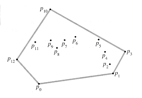
The convex hull of a set Q of points is the smallest convex polygon P for which each point in Q is either on the boundary of P or in its interior. We denote the convex hull of Q by CH(Q). Intuitively, we can think of each point in Q as being a nail sticking out from a board. The convex hull is then the shape formed by a tight rubber band that surrounds all the nails. Figure 6 shows a set of points and its convex hull.

In this section, we shall present two algorithms that compute the convex hull of a set of n points. Both algorithms output the vertices of the convex hull in counterclockwise order. The first, known as Graham's scan, runs in O(n lg n) time. The second, called Jarvis's march, runs in O(nh) time, where h is the number of vertices of the convex hull. As can be seen from Figure 6, every vertex of CH(Q) is a point in Q. Both algorithms exploit this property, deciding which vertices in Q to keep as vertices of the convex hull and which vertices in Q to throw out.

Figure 6 A set of points Q with its convex hull CH(Q) in gray.

There are, in fact, several methods that compute convex hulls in O(n lg n) time. Both Graham's scan and Jarvis's march use a technique called 'rotational sweep,' processing vertices in the order of the polar angles they form with a reference vertex. Other methods include the following.

In the incremental method, the points are sorted from left to right, yielding a sequence <p₁,p₂, . . . , p_n>. At the ith stage, the convex hull CH() of the i - 1 leftmost points is updated according to the ith point from the left, thus forming CH(). As Exercise 3-6 asks you to show, this method can be implemented to take a total of O(n lg n) time.

In the divide-and-conquer method, in (n) time the set of n points is divided into two subsets, one of the leftmost n points and one of the rightmost n points, the convex hulls of the subsets are computed recursively, and then a clever method is used to combine the hulls in O(n) time.

The prune-and-search method is similar to the worst-case linear-time median algorithm of Section 10.3. It finds the upper portion (or 'upper chain') of the convex hull by repeatedly throwing out a constant fraction of the remaining points until only the upper chain of the convex hull remains. It then does the same for the lower chain. This method is asymptotically the fastest: if the convex hull contains h vertices, it runs in only O(n lg h) time.

Computing the convex hull of a set of points is an interesting problem in its own right. Moreover, algorithms for some other computational-geometry problems start by computing a convex hull. Consider, for example, the two-dimensional farthest-pair problem: we are given a set of n points in the plane and wish to find the two points whose distance from each other is maximum. As Exercise 3-3 asks you to prove, these two points must be vertices of the convex hull. Although we won't prove it here, the farthest pair of vertices of an n-vertex convex polygon can be found in O(n) time. Thus, by computing the convex hull of the n input points in O(n lg n) time and then finding the farthest pair of the resulting convex-polygon vertices, we can find the farthest pair of points in any set of n points in O(n lg n) time.

Graham's scan

Graham's scan solves the convex-hull problem by maintaining a stack S of candidate points. Each point of the input set Q is pushed once onto the stack, and the points that are not vertices of CH(Q) are eventually popped from the stack. When the algorithm terminates, stack S contains exactly the vertices of CH(Q), in counterclockwise order of their appearance on the boundary.

Figure 7 The execution of GRAHAM-SCAN on the set Q of Figure 6. The current convex hull contained in stack S is shown in gray at each step. (a) The ordered polar angles of p₁,p₂, . . . , p₁₂ relative to p₀ and the initial stack S containing p₀, p₁, and p₂. (b)-(k) Stack S after each iteration of the for loop of lines 7-10. Dashed lines show nonleft turns, which cause points to be popped from the stack. In part (h), for example, the right turn at angle p₇p₈p₉ causes p₈ to be popped, and then the right turn at angle p₆p₇p₉ causes p₇ to be popped. (l) The convex hull returned by the procedure, which matches that of Figure 6.

The procedure GRAHAM SCAN takes as input a set Q of points, where |Q| 3. It calls the functions TOP(S), which returns the point on top of stack S without changing S, and NEXT TO TOP(S), which returns the point one entry below the top of stack S without changing S. As we shall prove in a moment, the stack S returned by GRAHAM SCAN contains, from bottom to top, exactly the vertices of CH(Q) in counterclockwise order.

GRAHAM-SCAN(Q)
let p₀ be the point in Q with the minimum y-coordinate,
or the leftmost such point in case of a tie
let p₁, p₂, . . . , p_m be the remaining points in Q,
sorted by polar angle in counterclockwise order around p₀
(if more than point has the same angle, remove all but
the one that is farthest from p₀)
top[S] 0
PUSH(p₀,S)
PUSH(p₁,S)
PUSH(p₂,S)
for i 3 to m
do while the angle formed by points NEXT-TO-TOP(S),
TOP(S), and p_i makes a nonleft turn
do POP(S)
PUSH(S,p_i)
return S

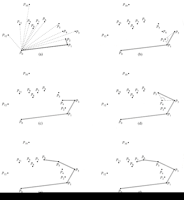
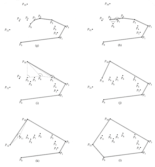
Figure 7 illustrates the progress of GRAHAM SCAN. Line 1 chooses point p₀ as the point with the lowest y-coordinate, picking the leftmost such point in case of a tie. Since there is no point in Q that is below p₀ and any other points with the same y-coordinate are to its right, p₀ is a vertex of CH(Q). Line 2 sorts the remaining points of Q by polar angle relative to p₀, using the same method--comparing cross products--as in Exercise 1-2. If two or more points have the same polar angle relative to p₀, all but the farthest such point are convex combinations of p₀ and the farthest point, and so we remove them entirely from consideration. We let m denote the number of points other than p₀ that remain. The polar angle, measured in radians, of each point in Q relative to p₀ is in the half-open interval [0, /2). Since polar angles increase in a counterclockwise fashion, the points are sorted in counterclockwise order relative to p₀. We designate this sorted sequence of points by p₁, p₂, . . . , p_m . Note that points p₁ and p_m are vertices of CH(Q) (see Exercise 3-1). Figure 7(a) shows the points of Figure 6, with the ordered polar angles of p₁, p₂, . . . , p₁₂ relative to p₀.

The remainder of the procedure uses the stack S Lines 3-6 initialize the stack to contain, from bottom to top, the first three points p₀, p₁, and p₂. Figure 7(a) shows the initial stack S. The for loop of lines 7-10 iterates once for each point in the subsequent p₃, p₄, . . . ,p_m) The intent is that after processing point p_i, stack S contains, from bottom to top, the vertices of CH() in counterclockwise order. The while loop of lines 8-9 removes points from the stack if they are found not to be vertices of the convex hull. When we traverse the convex hull counterclockwise, we should make a left turn at each vertex. Thus, each time the while loop finds a vertex at which we make a nonleft turn, the vertex is popped from the stack. (By checking for a nonleft turn, rather than just a right turn, this test precludes the possibility of a straight angle at a vertex of the resulting convex hull. This is just what we want, since every vertex of a convex polygon must not be a convex combination of other vertices of the polygon.) After we pop all the vertices that have nonleft turns when heading toward point p_i we push p_i onto the stack. Figures 7(b)-(k) show the state of the stack S after each iteration of the for loop. Finally, GRAHAM-SCAN returns the stack S in line 11. Figure 7(1) shows the corresponding convex hull.

The following theorem formally proves the correctness of GRAHAM SCAN

Theorem 2

If GRAHAM SCAN is run on a set Q of points, where |Q| 3, then a point of Q is on the stack S at termination if and only if it is a vertex of CH(Q).

Proof As noted above, a vertex that is a convex combination of p₀ and some other vertex in Q is not a vertex of CH(Q). Such a vertex is not included in the sequence p_l, p₂, . . . , p _m, and so it can never appear on stack S.

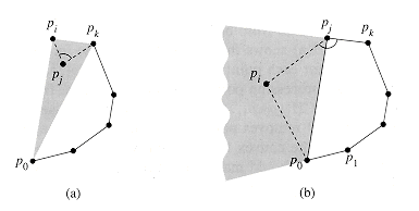
The crux of the proof lies in the two situations shown in Figure 8. Part (a) deals with nonleft turns, and part (b) deals with left turns.

We first show that each point popped from stack S is not a vertex of CH(Q). Suppose that point p_j is popped from the stack because angle p_kp_jp_i makes a nonleft turn, as shown in Figure 8(a). Because we scan the points in order of increasing polar angle relative to point p₀, there is a triangle with point p_j either in the interior of the triangle or on line segment . In either case, point p_j cannot be a vertex of CH(Q).

We now show that each point on stack S is a vertex of CH(Q) at termination. We start by proving the following claim: GRAHAM SCAN maintains the invariant that the points on stack S always form the vertices of a convex polygon in counterclockwise order.

The claim holds immediately after the execution of line 6, since points p₀, p₁, and p₂ form a convex polygon. Now we examine how stack S changes during the course of GRAHAM-SCAN. Points are either popped or pushed. In the former case, we rely on a simply geometrical property: if a vertex is removed from a convex polygon, the resulting polygon is convex. Thus, popping a point from stack S preserves the invariant.

Figure 8 The two basic situations in the proof of correctness of GRAHAM SCAN (a) Showing that a point popped from the stack in GRAHAM SCAN is not a vertex of CH(Q). If point p_j is popped from the stack because angle p_kp_jp_i makes a nonleft turn, then the shaded triangle contains point p_j Point p_j is therefore not a vertex of CH(Q). (b) If point p_i is pushed onto the stack, then there must be a left turn at angle p_kp_jp_i. Because p_i follows p_j in the polar-angle ordering of points and because of how p₀ was chosen, p_i must be in the shaded region. If the points on the stack form a convex polygon before the push, then they must form a convex polygon afterward.

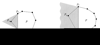
Before we consider the case in which a point is pushed onto the stack, let us examine another geometrical property, illustrated in Figures 9(a) and (b). Let P be a convex polygon, and choose any side of P. Consider the region bounded by and the extensions of the two adjacent sides. (Depending on the relative angles of the adjacent sides, the region may be either bounded, like the shaded region in part (a), or unbounded, like the shaded region in part (b).) If we add any point p_s in this region to P as a new vertex, with the sides replacing side , the resulting polygon is convex.

Now consider a point pi that is pushed onto S. Referring back to Figure 8(b), let p_j be the vertex on the top of S just prior to pushing pi, and let p_k be the predecessor of p_j on S. We claim that p_i must fall within the shaded region of Figure 8(b), which corresponds directly to the shaded regions of Figure 9. Because the angle p_kp_jp_i makes a left turn, p_i must be on the shaded side of the extension of . Because p_i follows p_j in the polar-angle ordering, it must be on the shaded side of . Moreover, because of how we chose p₀, point p_i must be on the shaded side of the extension of . Thus, p_i is in the shaded region, and therefore after p_i has been pushed onto stack S, the points on S form a convex polygon. This completes the proof of the claim.

At the end of GRAHAM SCAN, therefore, the points of Q that are on stack S form the vertices of a convex polygon. We have shown that all points not on S are not vertices of CH(Q) or, equivalently, that all vertices of CH(Q) are on S. Since S contains only vertices from Q and its points form a convex polygon, they must form CH(Q).

Figure 9 Adding a point in the shaded region to a convex polygon P yields another convex polygon. The shaded region is bounded by a side of and the extensions of the two adjacent sides. (a) The shaded region is bounded. (b) The shaded region is unbounded.

We now show that the running time of GRAHAM SCAN is O(n lg n), where n = |Q|. Line 1 takes(n) time. Line 2 takes O(n lg n) time, using merge sort or heapsort to sort the polar angles and the cross-product method of Section 1 to compare angles. (Removing all but the farthest point with the same polar angle can be done in a total of O(n) time.) Lines 3-6 take O(1) time. Because m n - 1, the for loop of lines 7-10 is executed at most n - 3 times. Since PUSH takes O(1) time, each iteration takes O(1) time exclusive of the time spent in the while loop of lines 8-9, and thus overall the for loop takes O(n) time exclusive of the nested while loop.

We use the aggregate method of amortized analysis to show that the while loop takes O(n) time overall. For i = O, 1, . . . , m, each point p_i is pushed onto stack S exactly once. As in the analysis of the MULTIPOP procedure of Section 18.1, we observe that there is at most one POP operation for each PUSH operation. At least three points--p₀, p₁, and p_m--are never popped from the stack, so that in fact at most m - 2 POP operations are performed in total. Each iteration of the while loop performs one POP, and so there are at most m - 2 iterations of the while loop altogether. Since the test in line 8 takes O(1) time, each call of POP takes O(1) time, and m n - 1, the total time taken by the while loop is O(n). Thus, the running time of GRAHAM SCAN is O(n lg n).

Jarvis's march

Jarvis's march computes the convex hull of a set Q of points by a technique known as package wrapping (or gift wrapping). The algorithm runs in time O(nh), where h is the number of vertices of CH(Q). When h is o(lg n), Jarvis's march is asymptotically faster than Graham's scan.

Figure 10 The operation of Jarvis's march. The first vertex chosen is the lowest point p₀. The next vertex, p₁, has the least polar angle of any point with respect to p₀. Then, p₂ has the least polar angle with respect to p₁. The right chain goes as high as the highest point p₃. Then, the left chain is constructed by finding least polar angles with respect to the negative x-axis.

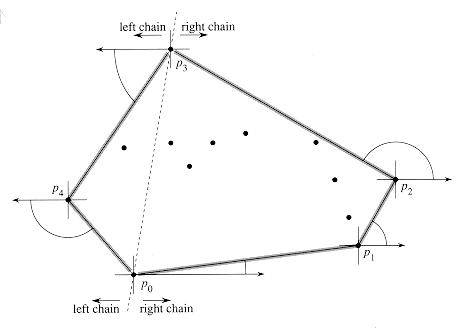
Intuitively, Jarvis's march simulates wrapping a taut piece of paper around the set Q. We start by taping the end of the paper to the lowest point in the set, that is, to the same point p₀ with which we start Graham's scan. This point is a vertex of the convex hull. We pull the paper to the right to make it taut, and then we pull it higher until it touches a point. This point must also be a vertex of the convex hull. Keeping the paper taut, we continue in this way around the set of vertices until we come back to our original point p₀.

More formally, Jarvis's march builds a sequence H = p₀, p₁, . . . , p_h-1 of the vertices of CH(Q). We start with p₀. As Figure 10 shows, the next convex hull vertex p₁ has the least polar angle with respect to p₀. (In case of ties, we choose the point farthest from p₀.) Similarly, p₂ has the least polar angle with respect to p_l, and so on. When we reach the highest vertex, say p_k (breaking ties by choosing the farthest such vertex), we have constructed, as Figure 10 shows, the right chain of CH(Q). To construct the left chain, we start at p_k and choose p_k+l as the point with the least polar angle with respect to p_k, but from the negative x-axis. We continue on, forming the left chain by taking polar angles from the negative x-axis, until we come back to our original vertex p₀.

We could implement Jarvis's march in one conceptual sweep around the convex hull, that is, without separately constructing the right and left chains. Such implementations typically keep track of the angle of the last convex-hull side chosen and require the sequence of angles of hull sides to be strictly increasing (in the range of 0 to 2 radians). The advantage of constructing separate chains is that we need not explicitly compute angles; the techniques of Section 1 suffice to compare angles.

If implemented properly, Jarvis's march has a running time of O(nh). For each of the h vertices of CH(Q), we find the vertex with the minimum polar angle. Each comparison between polar angles takes O(1) time, using the techniques of Section 1. As Section 10.1 shows, we can compute the minimum of n values in O(n) time if each comparison takes O(1) time. Thus, Jarvis's march takes O(nh) time.

Exercises

Prove that in the procedure GRAHAM SCAN, points p₁ and p_m must be vertices of CH(Q).

Consider a model of computation that supports addition, comparison, and multiplication and for which there is a lower bound of (n lg n) to sort n numbers. Prove that (n lg n) is a lower bound for computing, in order, the vertices of the convex hull of a set of n points in such a model.

Given a set of points Q, prove that the pair of points farthest from each other must be vertices of CH(Q).

For a given polygon P and a point q on its boundary, the shadow of q is the set of points r such that the segment is entirely on the boundary or in the interior of P. A polygon P is star-shaped if there exists a point p in the interior of P that is in the shadow of every point on the boundary of P. The set of all such points p is called the kernel of P. (See Figure 11.) Given an n-vertex, star-shaped polygon P specified by its vertices in counterclockwise order, show how to compute CH(P) in O(n) time.

In the on-line convex-hull problem, we are given the set Q of n points one point at a time. After receiving each point, we are to compute the convex hull of the points seen so far. Obviously, we could run Graham's scan once for each point, with a total running time of O(n² l g n). Show how to solve the on-line convex-hull problem in a total of O(n²) time.

Figure 11 The definition of a star-shaped polygon, for use in Exercise 3-4. (a) A star-shaped polygon. The segment from point p to any point q on the boundary intersects the boundary only at q. (b) A non-star-shaped polygon. The shaded region on the left is the shadow of q, and the shaded region on the right is the shadow of q'. Since these regions are disjoint, the kernel is empty.

Show how to implement the incremental method for computing the convex hull of n points so that it runs in O(n lg n) time.

4 Finding the closest pair of points

We now consider the problem of finding the closest pair of points in a set Q of n 2 points. 'Closest' refers to the usual euclidean distance: the distance between points p₁ = (x₁, y₁) and p₂ = (x₂, y₂) is . Two points in set Q may be coincident, in which case the distance between them is zero. This problem has applications in, for example, traffic-control systems. A system for controlling air or sea traffic might need to know which are the two closest vehicles in order to detect potential collisions.

A brute-force closest-pair algorithm simply looks at all the pairs of points. In this section, we shall describe a divide-and-conquer algorithm for this problem whose running time is described by the familiar recurrence T(n) = 2T(n/2) + O(n). Thus, this algorithm uses only O(n lg n) time.

The divide-and-conquer algorithm

Each recursive invocation of the algorithm takes as input a subset P Q and arrays X and Y, each of which contains all the points of the input subset P. The points in array X are sorted so that their x-coordinates are monotonically increasing. Similarly, array Y is sorted by monotonically increasing y-coordinate. Note that in order to attain the O(n lg n) time bound, we cannot afford to sort in each recursive call; if we did, the recurrence for the running time would be T(n) = 2T(n/2) + O(n lg n), whose solution is T(n) = O(n 1g² n). We shall see a little later how to use 'presorting' to maintain this sorted property without actually sorting in each recursive call.

A given recursive invocation with inputs P, X, and Y first checks whether |P| 3. If so, the invocation simply performs the brute-force method described above: try all pairs of points and return the closest pair. If |P| > 3, the recursive invocation carries out the divide-and-conquer paradigm as follows.

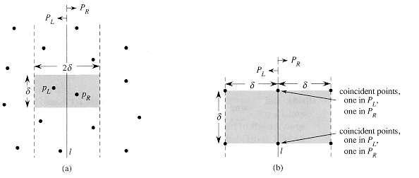
Divide: It finds a vertical line l that bisects the point set P into two sets P_L and P_R such that |P_L| = |P|/2, |P_R| = |P| /2, all points in P_L are on or to the left of line l, and all points in P_R are on or to the right of l. The array X is divided into arrays X_L and X_R, which contain the points of P_L and P_R respectively, sorted by monotonically increasing x-coordinate. Similarly, the array Y is divided into arrays Y_L and Y_R, which contain the points of P_L and P_R respectively, sorted by monotonically increasing y-coordinate.

Conquer: Having divided P into P_L and P_R, it makes two recursive calls, one to find the closest pair of points in P_L and the other to find the closest pair of points in P_R. The inputs to the first call are the subset P_L and arrays X_L and Y_L; the second call receives the inputs P_R, X_R, and Y_R. Let the closest-pair distances returned for P_L and P_R be _L and _R, respectively, and let = min(_L, _R).

Combine: The closest pair is either the pair with distance found by oneof the recursive calls, or it is a pair of points with one point in P_L and the other in P_R. The algorithm determines if there is such a pair whose distance is less than . Observe that if there is a pair of points with distance less than , both points of the pair must be within units of line l. Thus, as Figure 12(a) shows, they both must reside in the 2-wide vertical strip centered at line l. To find such a pair, if one exists, the algorithm does the following.

1. It creates an array Y', which is the array Y with all points not in the 2-wide vertical strip removed. The array Y' is sorted by y-coordinate, just as Y is.

2. For each point p in the array Y', the algorithm tries to find points in Y' that are within units of p. As we shall see shortly, only the 7 points in Y' that follow p need be considered. The algorithm computes the distance from p to each of these 7 points and keeps track of the closest-pair distance ' found over all pairs of points in Y'.

3. If ' < , then the vertical strip does indeed contain a closer pair than was found by the recursive calls. This pair and its distance ' are returned. Otherwise, the closest pair and its distance found by the recursive calls are returned.

Figure 12 Key concepts in the proof that the closest-pair algorithm needs to check only 7 points following each point in the array Y'. (a) If P_L P_L and P_R P_R are less than units apart, they must reside within a x 2 rectangle centered at line l. (b) How 4 points that are pairwise at least units apart can all reside within a x square. On the left are 4 points in P_L, and on the right are 4 points in P_R There can be 8 points in the x 2 rectangle if the points shown on line l are actually pairs of coincident points with one point in P_L and one in P_R

The above description omits some implementation details that are necessary to achieve the O(n 1g n) running time. After proving the correctness of the algorithm, we shall show how to implement the algorithm to achieve the desired time bound.

Correctness

The correctness of this closest-pair algorithm is obvious, except for two aspects. First, by bottoming out the recursion when |P| 3, we ensure that we never try to divide a set of points with only one point. The second aspect is that we need only check the 7 points following each point p in array Y'; we shall now prove this property.

Suppose that at some level of the recursion, the closest pair of points is p_L P_L and P_R P_R. Thus, the distance ' between P_L and P_R is strictly less than . Point p_L must be on or to the left of line l and less than units away. Similarly, p_R is on or to the right of l and less than units away. Moreover, p_L and p_R are within units of each other vertically. Thus, as Figure 12(a) shows, p_L and p_R are within a X 2 rectangle centered at line l. (There may be other points within this rectangle as well.)

We next show that at most 8 points of P can reside within this X 2 rectangle. Consider the X square forming the left half of this rectangle. Since all points within P_L are at least units apart, at most 4 points can reside within this square; Figure 12(b) shows how. Similarly, at most 4 points in P_R can reside within the X square forming the right half of the rectangle. Thus, at most 8 points of P can reside within the X 2 rectangle. (Note that since points on line l may be in either P_L or P_R, there may be up to 4 points on l. This limit is achieved if there are two pairs of coincident points, each pair consisting of one point from P_L and one point from P_R, one pair is at the intersection of l and the top of the rectangle, and the other pair is where l intersects the bottom of the rectangle.)

Having shown that at most 8 points of P can reside within the rectangle, it is easy to see that we need only check the 7 points following each point in the array Y'. Still assuming that the closest pair is P_L and P_R, let us assume without loss of generality that p_L precedes p_R in array Y'. Then, even if p_L occurs as early as possible in Y' and p_R occurs as late as possible, p_R is in one of the 7 positions following p_L. Thus, we have shown the correctness of the closest-pair algorithm.

Implementation and running time

As we have noted, our goal is to have the recurrence for the running time be T(n) = 2T(n/2) + O(n), where T(n) is, of course, the running time for a set of n points. The main difficulty is in ensuring that the arrays X_L, X_R, Y_L, and Y_R, which are passed to recursive calls, are sorted by the proper coordinate and also that the array Y' is sorted by y-coordinate. (Note that if the array X that is received by a recursive call is already sorted, then the division of set P into P_L and P_R is easily accomplished in linear time.)

The key observation is that in each call, we wish to form a sorted subset of a sorted array. For example, a particular invocation is given the subset P and the array Y, sorted by y-coordinate. Having partitioned P into P_L and P_R, it needs to form the arrays Y_L and Y_R, which are sorted by y-coordinate. Moreover, these arrays must be formed in linear time. The method can be viewed as the opposite of the MERGE procedure from merge sort in Section 1.3.1: we are splitting a sorted array into two sorted arrays. The following pseudocode gives the idea.

length[Y_L] length[Y_R] 0
for i 1 to length[Y]
do if Y[i] P_L
then length[Y_L] length[Y_L] + 1
Y[length[Y_L]] Y[i]
else length[Y_R] length[Y_R] + 1
Y[length[Y_R]] Y[i]

We simply examine the points in array Y in order. If a point Y[i] is in P_L, we append it to the end of array Y_L; otherwise, we append it to the end of array Y_R. Similar pseudocode works for forming arrays X_L, X_R, and Y'.

The only remaining question is how to get the points sorted in the first place. We do this by simply presorting them; that is, we sort them once and for all before the first recursive call. These sorted arrays are passed into the first recursive call, and from there they are whittled down through the recursive calls as necessary. The presorting adds an additional O(n lg n) to the running time, but now each step of the recursion takes linear time exclusive of the recursive calls. Thus, if we let T(n) be the running time of each recursive step and T'(n) be the running time of the entire algorithm, we get T'(n) = T(n) + O(n lg n) and

Thus, T(n) = O(n lg n) and T'(n) = O(n lg n).

Exercises

Professor Smothers comes up with a scheme that allows the closest-pair algorithm to check only 5 points following each point in array Y'. The idea is always to place points on line l into set P_L. Then, there cannot be pairs of coincident points on line l with one point in P_L and one in P_R. Thus, at most 6 points can reside in the x 2 rectangle. What is the flaw in the professor's scheme?

Without increasing the asymptotic running time of the algorithm, show how to ensure that the set of points passed to the very first recursive call contains no coincident points. Prove that it then suffices to check the points in the 6 (not 7) array positions following each point in the array Y'. Why doesn't it suffice to check only the 5 array positions following each point?

The distance between two points can be defined in ways other than euclidean. In the plane, the L_m-distance between points p₁ and p₂ is given by ((x₁ - x_2]^m _{+ (}y₁ - y₂)^m)^1/m. Euclidean distance, therefore, is L₂-distance. Modify the closest-pair algorithm to use the L₁-distance, which is also known as the Manhattan distance.

Given two points p₁ and p₂ in the plane, the L-distance between them is max(|x - x |, |y - y |). Modify the closest-pair algorithm to use the L-distance.

Problems

35-1 Convex layers

Given a set Q of points in the plane, we define the convex layers of Q inductively. The first convex layer of Q consists of those points in Q that are vertices of CH(Q). For i > 1, define Q_i to consist of the points of Q with all points in convex layers 1, 2, . . . , i - 1 removed. Then, the ith convex layer of Q is CH(Q_i) if and is undefined otherwise.

a. Give an O(n²)-time algorithm to find the convex layers of a set on n points.

b. Prove that (n lg n) time is required to compute the convex layers of a set of n points on any model of computation that requires (n lg n) time to sort n real numbers.

35-2 Maximal layers

Let Q be a set of n points in the plane. We say that point (x, y) dominates point (x', y') if x x' and y y'. A point in Q that is dominated by no other points in Q is said to be maximal. Note that Q may contain many maximal points, which can be organized into maximal layers as follows. The first maximal layer L₁ is the set of maximal points of Q. For i > 1, the ith maximal layer L_i is the set of maximal points in .

Suppose that Q has k nonempty maximal layers, and let y_i be the y-coordinate of the leftmost point in L_i for i = 1, 2, . . . ,k. For now, assume that no two points in Q have the same x - or y-coordinate.

a. Show that y₁ > y₂ > . . . > y_k.

Consider a point (x, y) that is to the left of any point in Q and for which y is distinct from the y-coordinate of any point in Q. Let Q' = Q .

b. Let j be the minimum index such that y_j < y, unless y < y_k, in which case we let j = k + 1. Show that the maximal layers of Q' are as follows.

If j k, then the maximal layers of Q' are the same as the maximal layers of Q, except that L_j also includes (x, y) as its new leftmost point.

If j = k + 1, then the first k maximal layers of Q' are the same as for Q, but in addition, Q' has a nonempty (k + 1)st maximal layer: L_k+1 = .

c. Describe an O(n lg n)-time algorithm to compute the maximal layers of a set Q of n points. (Hint: Move a sweep line from right to left.)

d. Do any difficulties arise if we now allow input points to have the same x- or y-coordinate? Suggest a way to resolve such problems.

35-3 Ghostbusters and ghosts

A group of n Ghostbusters is battling n ghosts. Each Ghostbuster is armed with a proton pack, which shoots a stream at a ghost, e radicating it. A stream goes in a straight line and terminates when it hits the ghost. The Ghostbusters decide upon the following strategy. They will pair off with the ghosts, forming n Ghostbuster-ghost pairs, and then simultaneously each Ghostbuster will shoot a stream at his or her chosen ghost. As we all know, it is very dangerous to let streams cross, and so the Ghostbusters must choose pairings for which no streams will cross.

Assume that the position of each Ghostbuster and each ghost is a fixed point in the plane and that no three positions are collinear.

a. Argue that there exists a line passing through one Ghostbuster and one ghost such the number of Ghostbusters on one side of the line equals the number of ghosts on the same side. Describe how to find such a line in O(n lg n) time.

b. Give an O(n² lg n)-time algorithm to pair Ghostbusters with ghosts in such a way that no streams cross.

35-4 Sparse-hulled distributions

Consider the problem of computing the convex hull of a set of points in the plane that have been drawn according to some known random distribution. Sometimes, the convex hull of n points drawn from such a distribution has O(n^1-) expected size for some constant > 0. We call such a distribution sparse-hulled. Sparse-hulled distributions include the following:

Points drawn uniformly from a unit-radius disk. The convex hull has (n^1/3) expected size.

Points drawn uniformly from the interior of a convex polygon with k sides, for any constant k. The convex hull has (1g n) expected size.

Points drawn according to a two-dimensional normal distribution. The convex hull has expected size.

a. Given two convex polygons with n₁ and n₂ vertices respectively, show how to compute the convex hull of all n₁ + n₂ points in O(n₁ + n₂) time. (The polygons may overlap.)

b. Show that the convex hull of a set of n points drawn independently according to a sparse-hulled distribution can be computed in O(n) expected time. (Hint: Recursively find the convex hulls of the first n/2 points and the second n/2 points, and then combine the results.)

Chapter notes

This chapter barely scratches the surface of computational-geometry algorithms and techniques. Books on computational geometry include those by Preparata and Shamos [160] and Edelsbrunner [60].

Although geometry has been studied since antiquity, the development of algorithms for geometric problems is relatively new. Preparata and Shamos note that the earliest notion of the complexity of a problem was given by E. Lemoine in 1902. He was studying euclidean constructions--those using a ruler and a straightedge--and devised a set of five primitives: placing one leg of the compass on a given point, placing one leg of the compass on a given line, drawing a circle, passing the ruler's edge through a given point, and drawing a line. Lemoine was interested in the number of primitives needed to effect a given construction; he called this amount the 'simplicity' of the construction.

The algorithm of Section 2, which determines whether any segments intersect, is due to Shamos and Hoey [176].

The original version of Graham's scan is given by Graham [91]. The package-wrapping algorithm is due to Jarvis [112]. Using a decision-tree model of computation, Yao [205] proved a lower bound of (n lg n) for the running time of any convex-hull algorithm. When the number of vertices h of the convex hull is taken into account, the prune-and-search algorithm of Kirkpatrick and Seidel [120], which takes O(n lg h) time, is asymptotically optimal.

The O(n lg n)-time divide-and-conquer algorithm for finding the closest pair of points is by Shamos and appears in Preparata and Shamos [160]. Preparata and Shamos also show that the algorithm is asymptotically optimal in a decision-tree model.