| CATEGORII DOCUMENTE |
| Bulgara | Ceha slovaca | Croata | Engleza | Estona | Finlandeza | Franceza |
| Germana | Italiana | Letona | Lituaniana | Maghiara | Olandeza | Poloneza |
| Sarba | Slovena | Spaniola | Suedeza | Turca | Ucraineana |
Beam Deflection
Introduction
A beam with a straight longitudinal axis subjected to transversal loads acting in its longitudinal plane of symmetry deforms and the resulting curve is called the deflection curve. In the previous lecture, the curvature of the deflection curve was used to determine the stress and strain distribution in the cross-section of a beam under the restrictions established for pure and nonuniform bending. In this lecture, the equation of the defection curve will be derived and consequently, the displacements at any point of the beam may be calculated. The calculation of beam deflections is an important part of structural analysis and design. The deflections are limited to prescribed tolerances imposed by the functionality of the particular structural element.
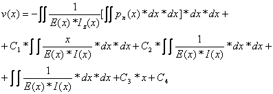
The cantilever beam pictured in Figure 1 deforms in its vertical plane of symmetry under the action of the exterior transversal loading.
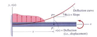
Figure 1 Example of Beam Deflection
The deflection curve and its slope
are mathematically represented by the real functions![]() and
and![]() ,
respectively. The vertical distance measured from a given point located on the
undeformed axis of the beam to the corresponding point located on the
deflection curve is called the transverse
displacement.
,
respectively. The vertical distance measured from a given point located on the
undeformed axis of the beam to the corresponding point located on the
deflection curve is called the transverse
displacement.
Qualitative Interpretation of the Deflection Curve
For the general case of
nonuniform bending the equation relating the bending moment ![]() with the radius of curvature
with the radius of curvature ![]() is:
is:
![]() (1)
(1)
where ![]() - modulus of elasticity;
- modulus of elasticity;
![]() -
moment of inertia about the horizontal centroidal axis of the cross-section;
-
moment of inertia about the horizontal centroidal axis of the cross-section;
![]() -
cross-section bending moment;
-
cross-section bending moment;
![]() -
radius of curvature of the deflection
curve.
-
radius of curvature of the deflection
curve.
Note: If the material is homogeneous linear elastic and the beam is of
uniform cross-section the product ![]() is called the flexural rigidity and is constant.
is called the flexural rigidity and is constant.
From the relation given by
equation (1), the deflection ![]() can be anticipated using the sign convention established
in Lecture 7 and re-plotted in Figure 2. The
moment diagram is always plotted at the beam side where the fibers are subjected
to tension, while the curvature center is placed on the opposite side. When
the bending moment is positive the deflection curvature is concave, while for
the negative bending moment the deflection curvature is convex. At the supports
the deflection must correspond to the prescribed support constraint condition. Locations
where the deflection curve changes from concave to convex, or vice versa, are
called inflection points.
can be anticipated using the sign convention established
in Lecture 7 and re-plotted in Figure 2. The
moment diagram is always plotted at the beam side where the fibers are subjected
to tension, while the curvature center is placed on the opposite side. When
the bending moment is positive the deflection curvature is concave, while for
the negative bending moment the deflection curvature is convex. At the supports
the deflection must correspond to the prescribed support constraint condition. Locations
where the deflection curve changes from concave to convex, or vice versa, are
called inflection points.
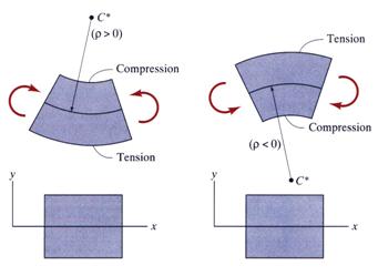
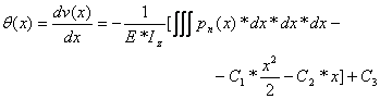
Figure 2 Sign Convention for Beams in Bending
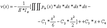
An example of qualitative interpretation of the deflection curve is shown in Figure 3. The moment diagram changes from positive to negative in the interval AB at point D. In between points A and D the moment is positive and the curvature center is located above the deflection curve. Between points D and B the moment diagram is negative and, thus, the curvature center is located below the deflection curve. The change in curvature takes place at point D, which is an inflection point. On the overhanging end BC, the moment is negative and the curvature is convex. Considering that at the supporting points the beam is constrained not to move vertically, the qualitative deflection diagram, as shown in Figure 3, can be sketched.
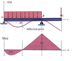
Figure 3 Example of Qualitative Interpretation of Deflection Curve
Differential Equations of the Deflection Curve
From Calculus it is known that the
slope of a real function at any particular point of its defined continuity
interval is the first derivative of the function. For the case in point, the
real function is represented by the beam displacement curve![]() .
Using the notation shown in Figure 1 the following relation is written:
.
Using the notation shown in Figure 1 the following relation is written:
![]() (2)
(2)
Under the assumption of small displacements, the first derivative is a very small value:
![]() (3)
(3)
consequently, the angle can approximate by its tangent:
![]() (4)
(4)
In Calculus the relation between the radius of curvature![]() and
the deflection
and
the deflection ![]() is
established as:
is
established as:
 (5)
(5)
Under the small displacement assumption (3), equation (5) can be simplified and written as:
![]() (6)
(6)
Substituting equation (6) into equation (1) yields the following equation:
![]() (7)
(7)
The moment-curvature equation, a second order differential equation, is obtained from equation (7) and expressed in the following standard form:
![]() (8)
(8)
where the notation ![]() is employed.
is employed.
Consider the differential
relation between the transverse loading and the cross-section stress resultants,
![]() and
and
![]() ,
previously obtained from the equilibrium of the beam infinitesimal volume
element:
,
previously obtained from the equilibrium of the beam infinitesimal volume
element:
![]() (9)
(9)
![]() (10)
(10)
where ![]() and
and
![]() are
the vertical shear force and the bending moment, respectively.
are
the vertical shear force and the bending moment, respectively.
Differentiating the moment-curvature equation (8) and using equations (9) and (10) the shear-deflection and load-deflection equations are obtained:
![]() (11)
(11)
![]() (12)
(12)
The load-deflection equation (12) is a forth-order differential equation.
If the beam is made from a homogeneous linear elastic material and has a constant cross-section in the continuity interval of the bending moment or transversal loading equations (8) and (12) became:
![]() (13)
(13)
![]() (14)
(14)
The general theory of differential equations with constant coefficients can be employed to obtain the solution of the second-order differential equation (8) and forth-order differential equation (12). The continuity intervals pertinent to the functions involved in these differential equations, the bending moment and transverse load, must be recognized in order for the integration process to be properly conducted.
Integration of the Moment- Curvature Differential Equation
Integration of the second-order
differential equation (8) on an interval of continuity for the bending moment![]() yields the following relations:
yields the following relations:
![]() (13)
(13)
![]() (14)
(14)
For the case of a beam with constant
bending stiffness ![]() ,
the integrals expressed in equations (13) and (14) may be simplified as
follows:
,
the integrals expressed in equations (13) and (14) may be simplified as
follows:
![]() (15)
(15)
![]() (16)
(16)
The integration constants ![]() and
and ![]() are calculated by imposing the boundary conditions of the specific
problem at hand.
are calculated by imposing the boundary conditions of the specific
problem at hand.
Integration of the Load-Deflection Differential Equation
Successive integration of the forth-order differential equation (12) in a continuity interval of the transverse loading function yields the following relations:
![]() (17)
(17)
![]() (18)
(18)
 (19)
(19)
 (20)
(20)
The integration constants![]() ,
,![]() ,
,
![]() and
and ![]() are calculated by imposing the boundary
conditions applicable to the specific problem.
are calculated by imposing the boundary
conditions applicable to the specific problem.
Note: The moment-curvature equation (8) can be used only if the bending moment variation is known, the case for statically determinate structures. The load-deflection curve equation (14) requires only that the variation of transverse load be known and, consequently, can be used for either statically determinate or indeterminate beams.
For the case of a beam with constant
bending stiffness ![]() ,
the integrals expressed in equations (17) through (20) may be considerably simplified
as follows:
,
the integrals expressed in equations (17) through (20) may be considerably simplified
as follows:
![]() (21)
(21)
![]() (22)
(22)
 (23)
(23)
 (24)
(24)
Boundary and Continuity Integration Conditions
As previously stated, the functions (15) though (21) obtained above, represent the general solutions. Only after the boundary conditions are imposed and the integration constants determined the solutions became representative for a specific case study.
The boundary conditions commonly encountered in the application of the equations (15) and (16) or equations (21) through (24) are presented in Table 1.
In general, the transverse load ![]() and
the bending moment
and
the bending moment ![]() functions
are described for a particular case by a number of continuity intervals.
Therefore, the continuity conditions
at the common ends of the intervals must be described in order for the
constants to be calculated. Each continuity interval is treated as an
independent interval and the boundary and continuity conditions are applied.
The most common continuity conditions are summarized in Table 2.
functions
are described for a particular case by a number of continuity intervals.
Therefore, the continuity conditions
at the common ends of the intervals must be described in order for the
constants to be calculated. Each continuity interval is treated as an
independent interval and the boundary and continuity conditions are applied.
The most common continuity conditions are summarized in Table 2.
Table 1 Boundary Conditions
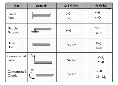
Table 2 Continuity Conditions
Examples
The methodology used in the application and integration of the moment-curvature (8) and load-deflection (14) differential equations is illustrated in examples 4.1 and 4.2, respectively.
Application of the Moment-Curvature Equation
The deflection curve is required
for a cantilever beam subjected to a concentrated force ![]() and a concentrated bending moment
and a concentrated bending moment ![]() both acting at the tip of the beam, point B. The
beam is characterized by a constant cross-section along its entire length, with
geometry and loading as shown in Figure 4.
both acting at the tip of the beam, point B. The
beam is characterized by a constant cross-section along its entire length, with
geometry and loading as shown in Figure 4.
![]() constant (25)
constant (25)
The corresponding reactions, ![]() and
and ![]() ,
are found using the equilibrium equations:
,
are found using the equilibrium equations:
![]() (26)
(26)
![]() (27)
(27)
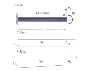
Figure 4 Cantilever Beam
The moment-curvature equation (8)
requires knowledge of the bending moment function and identification of the
continuity intervals. For the case in point, the bending moment ![]() diagram
is continuous on the entire length of the beam and is expressed as:
diagram
is continuous on the entire length of the beam and is expressed as:
![]() (28)
(28)
Using equation (28) in the moment-curvature equation (13), the problem specific differential equation is obtained:
![]() (29)
(29)
Integrating the differential equation (29) twice yields the following expressions for deflection and slope:
![]() (30)
(30)
![]() (31)
(31)
The integration constants ![]() and
and
![]() are
identified using the boundary conditions at point A:
are
identified using the boundary conditions at point A:
![]()
![]()
![]() (32)
(32)
![]() (33)
(33)
Solving the algebraic equations (32)
and (33) by substitution of equations (30) and (31) the integration constants ![]() and
and
![]() are
found as:
are
found as:
![]() (34)
(34)
![]() (35)
(35)
Substituting equations (34) and (35) into equations (30) and (31), the final deflection and slope expressions are obtained:
![]() (36)
(36)
![]() (37)
(37)
The maximum deflection value is obtained at the tip of the cantilever:
![]() (38)
(38)
and the corresponding rotation
![]() (39)
(39)
The deflection curve is a cubic (third-order) polynomial and is schematically plotted in Figure 5
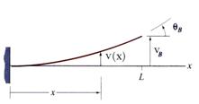
Figure 5 Deflection curve
Equations (38) and (39) may be written
for the case when only the concentrated force ![]() is considered:
is considered:
![]() (40)
(40)
![]() (41)
(41)
In the absence of the
concentrated force ![]() equations (38) and (39) become:
equations (38) and (39) become:
![]() (42)
(42)
![]() (43)
(43)
Application of the Load-Deflection Equation
The simply supported beam shown
in Figure 6 is subjected to a concentrated vertical force ![]() acting
at distance
acting
at distance ![]() from the fixed support A. The beam has a
constant flexural rigidity along its entire length.
from the fixed support A. The beam has a
constant flexural rigidity along its entire length.
![]() constant (44)
constant (44)
The reaction force and moment at point A are obtained by solution of the equilibrium equations:
![]() (45)
(45)
![]() (46)
(46)
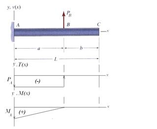
Figure 6 Cantilever Beam
The transverse load has two continuity intervals, AB and BC, and, consequently, the forth-order differential equation must be integrated for each one of them as:
![]() (47)
(47)
Using equation (47) in equations (21) through (24) yields the following:
![]() (48)
(48)
![]() (49)
(49)
![]() (50)
(50)
![]() (51)
(51)
![]() (52)
(52)
Equations (21) through (24) are written considering equation (52) as:
![]() (53)
(53)
![]() (54)
(54)
![]() (55)
(55)
![]() (56)
(56)
Eight (8) integration constants must be calculated. Four (4) boundary conditions (at points A and C) and four (4) continuity conditions (at point B) are employed. The boundary conditions are expressed as:
![]()
![]() (57)
(57)
![]()
![]()
![]() (58)
(58)
![]()
![]() (59)
(59)
![]()
![]() (60)
(60)
![]()
![]() (61)
(61)
![]()
![]() (62)
(62)
![]()
![]() (63)
(63)
![]()
![]() (64)
(64)
Solving the system of algebraic equations (57) through (64) the integration constants are calculated:
![]()
![]()
![]()
![]() (65)
(65)
![]()
![]()
![]()
![]() (66)
(66)
Substituting the integration constants (65) and (66) into equations (48) through (51) and (53) through (56), respectively, the variation of the shear force, bending moment, slope and deflection for each interval are obtained:
![]() (67)
(67)
![]() (68)
(68)
![]() (69)
(69)
![]() (70)
(70)
![]() (71)
(71)
![]() (72)
(72)
![]() (73)
(73)
![]() (74)
(74)
The deflection and slope at points B and C are:
![]() (75)
(75)
 (76)
(76)
![]() (77)
(77)
 (78)
(78)
|
Politica de confidentialitate | Termeni si conditii de utilizare |

Vizualizari: 6495
Importanta: ![]()
Termeni si conditii de utilizare | Contact
© SCRIGROUP 2024 . All rights reserved