| CATEGORII DOCUMENTE |
| Bulgara | Ceha slovaca | Croata | Engleza | Estona | Finlandeza | Franceza |
| Germana | Italiana | Letona | Lituaniana | Maghiara | Olandeza | Poloneza |
| Sarba | Slovena | Spaniola | Suedeza | Turca | Ucraineana |
RECONSTRUCTION AND flattening of the surface shoe last
The flattening of digitized surfaces is still very important in design of thin walled objects such as the airplane wings, parts of car bodies, textile products, and shoe uppers. Especially in shoe industry, the ability of quick respond to changing market needs is essential for successful competition. To give needed flexibility to a shoe designer, special CAD/CAM systems have been developed. Those systems are based on algorithms for surface reconstruction and surface flattening. In this article a fast algorithm for surface reconstruction and surface flattening is presented. Developable stripes are used to approximate a surface. In this way the surface can be flattened fast and without any distortions.
Key words: surface flattening, developable surfaces, pattern engineering, digitized surfaces, shoe design
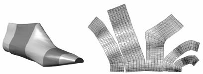
The needs on shoe market change today faster than ever. The shoe series are therefore smaller and the new shoe models have to be developed faster. The classical design of a new shoe is bound to the shoe last that is the form on which a shoe is constructed. The last gives the shoe a shape see Figure 1a). To construct the appearance of a new shoe, the style lines are drawn on the shoe last. The style lines are geodesic curves that partition the shoe last surface in the 3D patches which have to be flattened in the plane to get cutting model for shoe uppers manufacturing. The flattening of these patches is therefore a reverse engineering process to assembling the leather parts for the shoe upper. This process is expensive and requires a well-trained developer. To make the design process faster and the production of new series cheaper, special CAD/CAM systems are used. The final result obtained by all CAD systems for the shoe design is a flat pattern based on the style lines, drawn on the shoe last. To generate flat patterns, the shoe last has to be digitized.
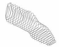
Basic modules in a modern CAD/CAM system for shoe design are those for last digitising and pattern engineering. The result of the last digitising phase is a cloud of points in 3D space which has to be approximated by a 3D surface composed of the set of independent triangles. Before such a surface can be flattened, the neighbouring relations between those triangles have to be established. Although algorithms for the surface reconstruction are very complex, the user is not aware of it, because they are part of the last digitising module. The result of the surface reconstruction, can be seen in figure 1.
Figure 1. a) Scattered points in 3D space, b) Surface reconstruction from scattered data
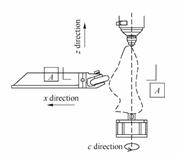
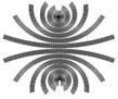
Currently, data acquisition can be divided into two categories: the contact measurement and noncontact measurement. Noncontact measurement is widely used in reverse engineering (RE). Although the noncontact measurement method has high efficiency and needs no offset probe radius, it is not accurate and is not suitable for certain measure types, such as shoe last measurement. This paper discusses only the asynchronous profile measurement method, in which, the measurement data are easily changed into NC machining path. The acquisition method of the surface profile measurement data is shown in fig. 2.
Owing to the fact that shoe last is a complicated closed free-form surface, it was clipped on the z axis; the probe moved along the direction of the x axis; and the probe head was driven by the cylinder. Using the raster rule record x axial coordinate, shoe last was driven by the thumb stall around the c axis. The measure rod reciprocated from the top to bottom in the direction of z axis; and the probe moved in the x axis to-and-fro in the drive of the cylinder, which pressed the probe to contact the shoe last surface while measuring. The measure trajectory is a space spiral curve, which contains uneven, dense, and large number of points. Hence it is difficult to construct the surface with common modeling methods.
![]()
Before becoming an NC program, shoe last surface measurement data should be reconstructed. It includes several essential technologies, such as the probe radius offset, the shoe last size magnification and shrinkage, the surface tool-path generation, and so on.
Currently, there are three types of surface structure methods in computational geometry [4]: one is based on B-spline or nonuniform rational B-spline (NURBS); the second is the triangle Bezier surface (TBS); and the third is the polyhedra method. The B-spline and the NURBS are the representations of the surface method that are currently adopted to a large extent in the commercialization of the CAD/CAM system. It occupies a strict request to the data point; the data form is distributed by the tensor, and it cannot be changed much. Otherwise the surface smoothness cannot be obtained satisfactorily.
In RE, the TBS modeling method has high speed and can be used to interpolate the arbitrary boundary. It is becoming a general method and getting more attention. On the basis of the shoe last profile measurement data character, this paper suggests a closed free-form surface triangle mesh modeling algorithm as follows.
Firstly, let us assume that the data points trace is a space spiral and each point is contextual. After knowing the data loop numbers, the locations of the data point are ensured completely. Let the data formats be , z,
where:
is the pole radius of the point,
is the pole angle
z is the length.
When adopting a measure method of angle increments, we have,
= 2n
where is the absolute angle of the point.
By the formula:
![]()
where the simple means getting an integer, we can obtain the turn number where this spot is located.
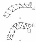
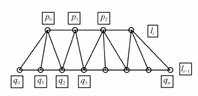
According to the actual measurement data distribution rule, as fig. 3 shows the data per loop links one by one in order; only adjacent two loop data points can link mutually. For the points in two adjacent loops, the existent condition is of two types:
1) the number of points in each loop is almost equal as shown in fig. 3(a);
2) the number of points in each loop is different as shown in fig. 3(b).
The links of all data points are as shown in Fig. 4.
Firstly, points p0 and q0 are linked. Only then two methods of linking can be chosen, either p0 and q1 or q0 and p1. According to the rule the triangle patch should be an isosceles triangle; we can judge which method is more reasonable. If p0 and q1 are more reasonable, q1p0 q is the best result. Then choosing q1 p0 as one side of the isosceles triangle, we repeat the above-mentioned process to get another result, q1 q p0. This process will go on till all data points in the spiral curve are linked.
To construct the vertex table and the triangle adjoin table, the following steps are involved:
Input all points into the vertex table;
Establish the original triangle mesh:
(i) choose two vertexes from the vertex table, and put them into the null table; (ii) select two vertexes Vi and Vi +1 from the next loop;
(iii) if V V Vi is more reasonable than V V Vi , then chose V V Vi and give the number of the angle; input two vertexes v1 and vi into the null TBL table; and input v2 into the head of the TBL table. Otherwise, choose V V Vi and generate the number of the angle; input two vertexes v1 and vi into the null TBL table; and input v2 into the head of the TBL table;
Main process of triangulation:
(i) get a point NN as the new vertex from the submit table according to two points in the TBL table, and seek the next circle, two neighbor points;
(ii) repeat the process of 2); (iii) end the process when the vertex table is null. Otherwise return to (i).
To confirm the validity of the algorithm in the article, we have carried out the triangle grid division to the shoe last model data, made the primitive data point to triangularize, and saved it as the standard Simon Torrance Limited (STL) document format. The file is 2.14 MB, the shoe last model size is 275 mmx85 mmx125 mm. When the output precision of the STL format is 0.01 mm, there are 2 678 triangles on the surface model as shown in Fig. 4(a). When the output precision of the STL format is 0.02 mm, there are 2 013 triangles as shown in Fig. 5. The example proved that the algorithm may produce the STL document fast and accurate.
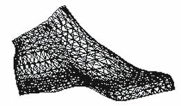
Figure 5 Shoe last triangle model
We have already mentioned that the result of surface digitising is a cloud of points in 3D space, where the groups of points lie in parallel planes the number of points in each plane is equal, see Figure 6. If line segments connect the points in each plane in the order given by the digitising process, the cross section curves ci, i =1,2, .N-1, are generated. After the cross section curves are determined, the surface construction can start. Let cs= cs(u) and cf = cf(u) be two cross section-guiding curves, where u and u are parameters of both curves. The equation of ruled surface defined by the curves cs and cf is given by [Gurunathan 1987].
After the surface is reconstructed, it has to be unrolled to the plane. Unrolling of the developable surface is, in fact, mapping of the 3D quadrangles into the plane, where geodesic distances are preserved. The mapping process must be fast and accurate. The quadrangles constructed in the plane must have the same length as the original 3D quadrangles. It turns out that the quadrangle construction is closely connected with the calculation error. Since calculation errors are accumulated and if the developable stripe consists of many quadrangles, the final error cannot be ignored. Therefore, we have to use the construction method presented in Kolmanic 2002. Flattening of the developable stripe is finished after all the quadrangles of the flat pattern depends upon the primary direction of flattening and the starting position. In our case the primary flattening direction has been u. Each quadrangle has been constructed independently from its neighbor and then translated and rotated in order to preserve the neighboring relation. The results of surface reconstruction and surface flattening are presented in the next section.
In this section we present the result of surface reconstruction and surface flattening on two test objects.
 A lot of time was designated to the study of
existing methods for the surface flattening and the generation of developable
surfaces. Since the flat pattern generation is an old and widespread problem,
many methods exist that try to solve this problem since the first attempts can
be found already in 1971. The surface can be unfolded to the plane without any
distortion only if the surface is developable. In other case, the distortions
like overlapping and tearing appear in the pattern.
A lot of time was designated to the study of
existing methods for the surface flattening and the generation of developable
surfaces. Since the flat pattern generation is an old and widespread problem,
many methods exist that try to solve this problem since the first attempts can
be found already in 1971. The surface can be unfolded to the plane without any
distortion only if the surface is developable. In other case, the distortions
like overlapping and tearing appear in the pattern.
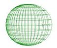
 If the distortions in the flat pattern are
too large, the pattern is unusable. But even, if the surface is not
developable, the flattening process can generate an usable pattern without any
additional efforts. Such surface is for example a sphere, whose flat pattern is
valid irrespective of the flattening method we use (see Figure 5).
If the distortions in the flat pattern are
too large, the pattern is unusable. But even, if the surface is not
developable, the flattening process can generate an usable pattern without any
additional efforts. Such surface is for example a sphere, whose flat pattern is
valid irrespective of the flattening method we use (see Figure 5).
![]()
The research on surface flattening has been continued to present days. Some of the methods for surface flattening were implemented in SURFMOD 3.0, for the others, the independent applications were developed. The example of the surface reconstruction of the shoe last from the scattered data obtained by a 3D scanner can bee seen in Figure 1.
This is especially true by designing shoes, where the shape of a shoe upper is defined by a shoe last. Therefore FlattGen enables the user to select only a part of the object to be flattened (see Figure 6).
In this article we have presented the new method for reconstruction and flattening of digitized surfaces, which is based on the divide-and conquer strategy by approximation of the surface with developable stripes.
It can effectively carry on the data processing, restructure surface to the profile scanning survey data, and enhance the product modeling efficiency. However, the technology such as surface structure based on the Bzier surface, needs to be studied further.
The method is fast but it cannot be used for reconstruction of objects with holes. To use the method in CAD systems for shoe design, the method for style lines mapping has to be developed first and the flattening method has to be modified to use those lines.
Acknowledgements: The paper is within the research activities of the CNMP programme INOSOC and BIOTECH, ctr. 106/006 and 41064/2007.
Azariadis, P., Asparagathos, N. (1997), Design of Plane Developments of Doubly Curved Surfaces, Computer-Aided Design, Vol. 29, No. 10, pp. 675685.
Bennis, C., Vezien, J. M., Inglesias, G. (1991), Piecewise surface flattening for non-distorted texture mapping, Computer Graphics, Vol. 25, No. 4, , pp. 237246.
Driscu, M., Mihai, A. (2008),
Approximated the cloud of the shoe last point by a set of developable stripes,
TMCR,
Driscu, M., Mihai, A. (2008),
Construct the surface of the shoe last by triangle meshes, TMCR,
Kos, G. (2001), An algorithm to triangulation surface in 3D using unorganized and point clouds, Computing, 14 (Supp1): 219232.
Ruqiong, L.I., Guangbu, L. I., Wang Y. (2007), Closed surface modeling with helical line measurement data, Higher Education Press and Springer-Verlag .
Yokoya, N., Levine, M.D. (1989), Range image segmentation based on differential geometry: a hybrid approach, IEEE Trans. on Pattern Anal Machine Intel, 11(6): 643649.
|
Politica de confidentialitate | Termeni si conditii de utilizare |

Vizualizari: 2797
Importanta: ![]()
Termeni si conditii de utilizare | Contact
© SCRIGROUP 2024 . All rights reserved