| CATEGORII DOCUMENTE |
| Bulgara | Ceha slovaca | Croata | Engleza | Estona | Finlandeza | Franceza |
| Germana | Italiana | Letona | Lituaniana | Maghiara | Olandeza | Poloneza |
| Sarba | Slovena | Spaniola | Suedeza | Turca | Ucraineana |
SuperPro Designer
User's Guide for the
Demonstration Version
Welcome to the functional demonstration of SuperPro Designer. SuperPro Designer is a superset of our Pro-Designer series tools that currently include BatchPro Designer, BioPro Designer and EnviroPro Designer. All four products share the same features (in terms of simulation, economic evaluation, throughput analysis, environmental impact assessment, communication with other popular software, etc.) and use the same interface but they differ in the list of modeling units; BatchPro and BioPro Designer include models mainly for specialty chemicals, biochemicals, pharmaceuticals, food, product formulation, and packaging processes. EnviroPro Designer includes models primarily for water and wastewater treatment, waste recycling, waste disposal, and air pollution control processes. SuperPro Designer is a superset of BatchPro and EnviroPro and can facilitate concurrent design and evaluation of chemical manufacturing and environmental processes. The table on the next page shows the current distribution of unit procedure models.
The Pro-Designer software family provides process simulation, comprehensive economic evaluation, advanced throughput analysis, process scheduling, and environmental impact assessment capabilities (including rigorous VOC emission calculations) in a single environment. These capabilities allow you to quickly identify process bottlenecks, reduce capital and operating costs, decrease time-to-market, increase tech transfer efficiency, perform accurate economic analyses, and more. Furthermore, the combination of manufacturing and environmental unit operation models in the same package enables the user to practice waste minimization via pollution prevention as well as pollution control.
This demo version offers you unrestricted access to all the features of SuperPro Designer except the ability to save your work. When you use SuperPro Designer, you will be joining a large group of scientists and engineers in companies like ADM, Akzo Nobel (Holland), Amersham Pharmacia Biotech, Baxter, Bayer, Borregaard (Norway), Bristol-Myers Squibb, CRAB (Italy), Cabot, Cargill, Development Center for Biotechnology (Taiwan), DSM (Holland and Spain), Du Pont, Eli Lilly, Fluor Daniel, Genentech, Genetics Institute, Gist-brocades (Holland and Mexico), Hemosol (Canada), Kraft, Kvaerner Process, Merck, Novo Nordisk (Denmark), Orsan / Amylum (France), Pfizer, Pliva (Croatia), Procter & Gamble, Ranbaxy (India), R.J. Reynolds, Rhone Poulenc Rorer (France), RTP Pharma (Canada), Sanofi (France and USA), Schering-Plough, SmithKline Beecham, Snamprogetti, SINTEF (Holland), Sumsung (Korea), U.S. DOA, DOD, DOE, etc. (just to name a few) in the U.S. and abroad who already are employing our technology to design new processes or improve the performance of existing ones.
SuperPro Designer for Windows has been designed and programmed with the latest tools and techniques, providing speed and ease of use without sacrifice of detail or accuracy. Following are some of the key features of SuperPro Designer:
Intuitive graphical user interface.
Complete simulation facilities including mass and energy balances as well as equipment sizing.
Throughput analysis and debottlenecking.
Models for over 120 unit procedures used in the process and environmental industries. Please refer to the first table that follows for a list of these unit procedures. Each unit procedure can contain a series of operations.
Thorough process economics.
Process scheduling of batch operations, including Gantt charts for equipment utilization and unit procedure tracking.
Resource tracking for utilities, labor, and raw materials as a function of time.
Rigorous VOC emission calculations and environmental impact assessment.
Extensive databases of process equipment, chemical components, and construction materials.
Compatibility with a variety of graphics, spreadsheet and word processing packages.
Advanced hypertext help facility.
Module for enhancing appearance of PFDs with visual objects.
OLE-2 support.
We at Intelligen are confident that after you become familiar with the facilities of SuperPro Designer, you'll find it to be one of the most valuable additions to your team's toolbox.
The concept of Unit Procedures is a new feature of version 4.0. A Unit Procedure is a set of operations that take place sequentially in a piece of equipment. For instance, a unit procedure that takes place in a reactor vessel may include: Charge material A, Heat, Charge material B, Agitate, React, Charge extraction solvent, Extract (Phase Split), Transfer Out bottom phase, Transfer Out top phase, etc. This set of operations is displayed on the PFD with a single reactor icon. Similarly, a unit procedure that takes place in a fermentor may include: Charge carbon source, Charge nutrients, Sterilize, Ferment, Transfer broth to surge tank, CIP, etc. The concept of unit procedures enables the user to model batch processes in great detail. The table that follows provides a complete list of unit procedure models.
Most previous unit
operations have been converted into unit procedures in version 4.0. As a
result, the old batch unit operations can be represented in version 4.0 in much
greater detail. For instance, the old Nutsche Filtration unit operation is now
represented with a Nutsche Filtration procedure that includes the following
operations: Filtration,
Several previous unit operations have become operations that are available in certain unit procedures. For instance, previous unit operations for batch reaction, fermentation, crystallization, extraction, etc. are now operations available in the context of Vessel Procedures.
A number of new operation models have been implemented that function in the context of certain unit procedures. For instance, in the content of Vessel Procedures, the list of new operation models includes: Charge, Transfer In, Transfer Out, Heat, Cool, Distill, Gas Sweep, Purge/Inert, Evacuate, Pressurize, Vent, Agitate, Hold, Clean In Place (CIP), and Sterilize In Place (SIP).
Unit Procedures in Continuous Processes If you deal with continuous processing steps in continuous flowsheets, then unit procedures become identical to the old unit operations. In such situations, all interface features that are reminiscent of unit procedures are hidden so that unit procedures can be truly perceived as unit operations by the user.
The SuperPro Designer demonstration version (as well as the full version) is written in Visual C++ using object oriented technology and runs on any PC that runs Windows 95 (or later) or Windows NT 4.0 (or later). It requires a minimum of 32 MB or RAM and 40 MB of hard disk space
(B: available in BatchPro/BioPro, E: available in EnviroPro. All models are available in SuperPro.)
|
Batch Vessel Procedures In a Stirred-Tank Reactor In a Stirred-Tank Fermentor (B) In an Air-Lift Fermentor (B) Continuous Reaction In a CSTR (stoichiometric, kinetic, or equilibrium) In a PFR (stoichiometric or kinetic) In a Fermentor (stoichiometric or kinetic) Heat Sterilization (B) Environmental Reaction Aerobic BioOxidation (E) Trickling Filtration (E) Anoxic Reaction (E) Anaerobic Digestion (E) Neutralization (E) Wet Air Oxidation (E) Incineration (E) Phase Separation Centrifugal Extraction (B) Differential Extraction (B) MixerSettler Extraction (B) Continuous Distillation (B) Batch Distillation (B) Flash (B) Condensation Continuous Crystallization (B) Absorption/Stripping Activated Carbon Adsorption Decantation Solid / Gas Separation Electrostatic Precipitation (E) Baghouse Filtration (E) Gas Cyclone Air Filtration Chromatography Gel Filtration (B) Packed Bed Adsorption (B) Expanded Bed Adsorption (B) Ion Exchange for Demineralization (E) Storage A wide variety of storage and blending tanks, including Silos and Hoppers for |
Solid / Liquid Separation Membrane Microfiltration (B) Membrane Ultrafiltration (B) Diafiltration (B) Reverse Osmosis DeadEnd Filtration Nutsche Filtration (B) Plate & Frame Filtration Rotary Vacuum Filtration (B) Granular Media Filtration (E) Belt Filtration (E) Basket Centrifugation (B) Bowl Centrifugation (B) Disk-Stack Centrifugation (B) Decanter Centrifugation Centritech Centrifugation (B) Hydrocyclone (B) Clarification / Thickening (E) Flotation (E) Oil Separation (E) Drying/Evaporation Freeze Drying (B) Tray Drying (B) Fluid Bed Drying (B) Spray Drying (B) Drum (B) Rotary Drying (B) Multi-Effect Evaporation (B) Sludge Drying (E) Product Formulation and Packaging Extrusion / Molding / Assembly (B) Trimming / Filling / Tableting (B) Boxing / Labelling / Printing (B) Transportation Land / Sea / Air (B) Other Models Generic Boxes Pumps / Compressor / Fan / Blower Conveyors (Screw, Belt, Pneumatic) (B) Bucket Elevator Homogenization (High Pressure and Bead Mill) (B) Flow Mixing / Splitting Component Splitting |
Before following the procedures below, make sure your system meets the requirements outlined in the preceding section.
Installation from a CD
Insert the CD into your CD-ROM drive to open the installation program. Follow the on-screen instructions to finish installing the functional demo of SuperPro Designer. If the installation program does not open automatically, locate and run the installation script (Setup.exe) that is available on the CD.
Installation from Downloaded Files
Locate and run the installation script (Setup.exe). It is part of the Demo1 file.
Installation from Diskettes
Insert Diskette 1 into a 3.5 inch floppy drive. From the Start button, select Run, and type in the following: a:Setup. Then click OK or hit ENTER. Alternatively, from Windows Explorer, display the contents of Diskette 1 and double click on Setup.exe.
As part of the installation process, the setup program will create a program group in the Start Button and include in it icons to run the program, the programs on-line Help, the ReadMe file and the examples.
![]()
The SuperPro Designer menu is similar to that of many MS Windows applications. An explanation of the menu options follows.
File
New - Create a new design case document.
Open - Open an existing design case document.
Close - Closes an open design case document.
Save - Not implemented in the demonstration system.
Save As - Not implemented in the demonstration system.
Drawing Size - Sets the page size and the drawing size for this flowsheet. Also, allows you to change other printer-specific settings.
Print - Prints a document.
Print Preview - Displays the document on screen as it would appear printed.
Last four files opened.
Export Items to Metafile - Export the selected objects of a flowsheet drawing in a metafile picture format (wmf format) so that it can later be imported by any graphics or word processing program that can read wmf format files.
Export Reports to Excel... - Export the reports to Excel files (tab-delimited ASCII files).
Exit - Exits SuperPro Designer
Edit
Cut - Deletes data from the document and moves it to the clipboard.
Copy - Copies data from the document to the clipboard.
Paste - Pastes data from the clipboard into the document.
Paste Special - Pastes data from the clipboard either as a picture or as an object that is still associated with the application that created it. The data can either be linked or embedded into Pro-Designers flowsheet.
Clear - Clears (irreversibly deletes) the selected items.
Clear All - Clears (irreversible deletes) all items of the current flowsheet.
Select All - Selects all the items in the current flowsheet.
Refresh - Redraws the entire flowsheet (refreshes the screen).
Flowsheet Options View and update general data pertaining to the flowsheet.
Unit Procedure Options View and update the data for a selected unit procedure.
Stream Options View and update the data for a selected material stream.
Visual Object Options Reshape visual object.
Text Options Edit text.
Insert new Object Copies a previously created OLE into the flowsheet.
Links Edit linked objects.
Object Activate embedded or linked object.
Unit Procedures - Provides choices of process steps (unit procedures) to add to the flowsheet. Refer to the table in Chapter 1 for a list of unit procedure models.
Tasks
Set Mode of Operation - Set the operation mode of the plant to either batch or continuous.
Register Components and Mixtures - Select the pure chemical components and the stock mixtures for the design case and optionally edit their properties.
Recipe Scheduling Information - Presents a dialog that allows you to edit the scheduling parameters of the production campaign. This dialog is only active when the plant mode is batch.
Gantt Charts - View and edit the scheduling information for your process in the form of a Gantt chart. One type of Gantt chart shows the unit procedures and operations, and another Gantt chart displays equipment utilization. Single or multiple batches can be displayed for either type of chart. This option is only active if the plants mode is batch.
Solve M&E balances - Solve the material and energy balances around the entire process.
Generate Stream Report - Generate and save in a file information about raw material requirements as well as information about all the streams in the flowsheet.
Revenue, Raw Material, and Waste Streams - Characterize input and output streams as revenue, raw material and waste; provide information about purchase cost, selling cost and / or waste treatment cost for waste streams.
Perform Economic Calculations - Perform economic analysis for the entire process. Will recalculate all economic parameters (capital cost, annual operating cost, ROI, etc.).
Generate Economic Evaluation Report (EER) - Generate and save in a file all economic figures and profitability indices for this process.
Generate Itemized Cost Report (ICR) - Generate and save in a file operating cost data reported on a per-section basis.
Generate Throughput Analysis Report (THR) - Generate and save in a file information about equipment capacity utilization and the potential for throughput increase without installation of additional equipment.
Generate Environmental Impact Report (EIR) - Generate and save in a file information about the waste that is generated by an integrated facility.
Generate Emissions Report (
Generate Input Data Report (IDR) Generate and save in a file information about the input data and the default values in the current design case.
Adjust Plant Throughput - Scale the throughput of a process by a specified factor.
View
Resource Chart Display utilization of ingredients, heat transfer agents, power, and labor as a function of time for single and multiple batches.
Executive Summary - Display key production and economic evaluation data.
Main Toolbar - Toggle the main toolbar display.
Status Bar - Toggle the status bar display.
Visual Objects Toolbar - Toggle the visual objects toolbar display.
Sections Toolbar - Toggle the sections toolbar display.
Window
Duplicate - Duplicate the current window without affecting the data.
Cascade - Display all windows as overlapping.
Tile - Display all windows as tiled.
Arrange Icons - Arrange icons if more than one flowsheet is open.
Select among the open flowsheets.
Databanks
Pure Components - Add or edit pure chemical components.
Stock Mixtures - Add or edit stock mixtures.
Construction Materials - Add or edit construction materials and factors.
Heat Transfer Agents - Add or edit heating or cooling agents.
Edit Databank Location - Specify a new location for all databank (.db) files.
Help
Help Topics - Offers you a table of contents for the entire help system.
Index - Offers you an index to topics on which you can get help.
Using Help - Presents helpful tips on how to use the on-line help system.
About - Displays the version number of this application.
Toolbar Buttons without Menu Equivalents
Select Mode ![]()
When this button is pushed, the system is in select mode. In this mode, you can
select unit procedures and streams by clicking on them. All selected objects
can be moved and deleted. Unit procedures can also be cut, copied, and pasted
in another place within the same flowsheet or another flowsheet created by the
program.
Connect Mode ![]()
When this button is pushed, the system is in connect mode. In this mode, you can easily connect unit
procedures by drawing process streams. When the system is in connect mode, the
cursor changes to a characteristic shape indicating that mouse clicks will be
interpreted specially. You cannot select
or drag icons, bring up right-click menus etc. while in connect mode. In order to cancel the drawing of a stream,
simply hit ESC.
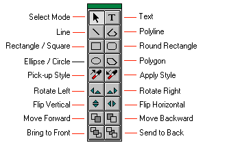
Using the above toolbar, the user can add to the flowsheet the following visual elements:
lines, polylines, rectangles/squares, round edge rectangles, ellipses/circles, polygons, and text.
The visual elements can be used to enhance the appearance of a process flow diagram. For instance, you may want to surround a certain section of the flowsheet by a rectangular boundary and assign it a name, since it represents a particular sub-section of the entire plant (e.g., the raw materials preparation). In other cases, the designer of a particular flowsheet may wish to comment on certain steps, so s/he may want to place some text right under a particular step. The visual elements have no effect on the physico-chemical transformations occurring in a process flowsheet.
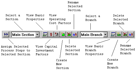
The concepts of flowsheet sections and branches facilitate reporting of results for costing, economic evaluation, raw material requirements, and throughput analysis of integrated processes. A flowsheet section is a group of processing steps that have something in common. For instance, typical sections in a flowsheet describing a biochemical plant might include the following: raw material preparation, fermentation, primary recovery, product isolation, final purification, product formulation, and packaging. A flowsheet branch is a set of flowsheet sections that have something in common. For instance, in a complicated, multi-step chemical synthesis (quite common for synthetic pharmaceuticals and agrichemicals), one may want to distinguish between the main path and the side synthesis paths (frequently performed by toll manufacturers). All parameters related to sections and branches of a flowsheet can be accessed and modified through the toolbar that is shown above.
In this section, we will guide you through the steps of creating a simple design case. The example process we will use illustrates the key initialization steps involved with the creation of any type of flowsheet. Thus, regardless of which industry you are in, you should read through this example to become familiar with the basic steps of modeling processes using any member of the Pro-Designer family (BatchPro, EnviroPro, BioPro, and SuperPro Designer) of simulation tools. In the rest of the chapter, references to SuperPro can be interchanged with any other member of the Pro-Designer family.
The steps listed below summarize the process of developing a design case with SuperPro. These steps are explained in much greater detail in the remainder of this chapter.
Initialize the flowsheet using the first three items of the Tasks menu: Set Mode of Operation, Register Components & Mixtures, and if the mode of operation is batch, Recipe Scheduling Information.
Build a flowsheet by selecting the desired procedures from the Unit Procedures menu. Switch to Connect Mode to draw the streams and connect the process steps.
Add operations, such as Charge, Agitate, Heat, React, etc. to each unit procedure (this applies to batch procedures only). Different unit procedures have different operations available to them. After the desired operations have been added, initialize all operations and streams.
Complete the analysis of the flowsheet using the remaining items of the Tasks menu: Solve M&E Balances, Generate Stream Report, supply Revenue, Raw Material and Waste Stream data, Perform Economic Calculations, Generate Economic Evaluation Report, etc. Other analyses may be optionally performed. Use the View menu to see the results of the analyses.
To begin working on a new flowsheet, simply open SuperPro Designer either by selecting it from your Start Menu or by double-clicking the Designer.exe application file in the SuperPro folder of your hard drive. After the program boots up, the following dialog box will appear:
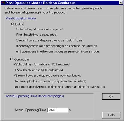
This dialog box allows you to set the primary mode of operation and the annual operating time for the new flowsheet. SuperPro Designer can model process plants that operate in batch, continuous, or mixed modes. You can also use the Tasks: Set Mode of Operation menu item to change the mode of operation at any time. Please note that SuperPro allows you to have continuous unit procedures in a batch flowsheet as well as batch (cyclical) procedures in a continuous flowsheet. Furthermore, when the operating mode of the entire plant is set to batch, all stream flows are displayed on a per-batch basis, as opposed to on a per-hour basis. For plants operating continuously, no scheduling information is necessary. At this point, please select Batch as the Plant Operation Mode for the example process which you will create.
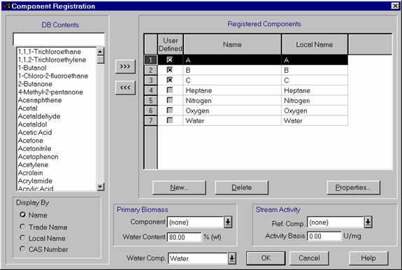
All the components that will be used in a design case must be specified. Many of these components may be selected from the component library in SuperPro Designer. To register components (in other words, to add them to your design case), choose the menu command Tasks: Register Components & Mixtures: Pure Components. This will activate the dialog shown below.
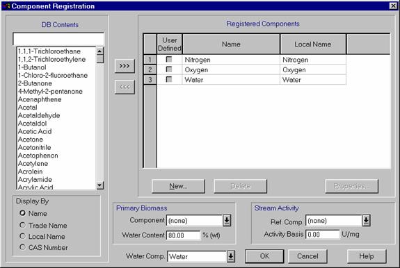
The Component Registration dialog.
By default, nitrogen, oxygen, and water are always registered as pure components in new processes. For this example process, you will need to add heptane to the list of registered components as well. To add heptane, you can either scroll down to it in the pure component database list on the left, or you can begin typing heptane in the box above the list and the database will automatically scroll to the correct location. Next, use the >>> button to add heptane to the Registered Components list for this flowsheet. Alternatively, you may double click on heptane in the database listing and it will be added to your list of Registered Components.
If a component does not appear in the library, you should use the 'New' button to add it. For this process, you will need to create three new components: A, B, and C. These components will represent the reactants and products of a simple reaction. To add component A to your database, click the New button and fill in the letter A for the Name, CAS Number, etc. (Note as far as the program is concerned, you do not have to have correct CAS Numbers, Formulas, etc. You just need to have something written in each of these six fields. The Local name is the one that appears in the reports and all the input/output dialog windows of the program.) Notice that at the bottom of this dialog box, you can choose to either initialize the physical properties to zero or copy them from some other component (see figure below.)
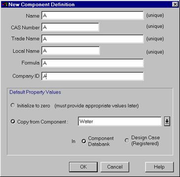
The New Component Definition dialog box.
For this example, simply click OK to copy the property values for component A from water. In general, it is recommended that you copy the properties of a new component from some other component as opposed to initializing them to zero. If you initialize the properties to zero, you must enter valid numbers for density, heat capacity, and many other properties before any simulations can be performed. On the other hand, copying the properties from another component allows you to do less editing since many of the physical properties will be the same (or very close).
After you have added component A to your list of registered components, follow the same steps to add components B and C. When you have completed this, you should edit some of the properties of these components. To access the basic properties of component A, select its line by clicking on the corresponding number on the left-most column of the table (e.g., number 1 for component A in the figure below) and then click on the Properties button. This brings up another dialog window which allows you to view and edit the physical and environmental properties of component A as well as its cost data and regulatory information.
For the purposes of this example, the only physical parameter we will be concerned with is the molecular weight (MW). For component A, please change the MW to 150 (as shown in the figure below). In addition, please go to the Economics tab, specify a purchase price of $10/kg, and press OK.
Next, please visit the Properties dialog for component B (by clicking on line 2 and then clicking the Properties button) and enter a MW of 25 and a purchase price of $15/kg. Finally, enter a MW of 175 and a selling price of $200/kg for component C. This completes your initialization of components for our example.
Notes:
1) If you need to delete a component from the Registered Components listing, click on the corresponding number on the left-most column of the table (e.g., number 1 for component A) and then click the Delete button.
2) If you wish to add components which you have edited or created to the permanent SuperPro database (so that you can access these components in future design case files), highlight the component by clicking on the corresponding number on the left-most column of the table (e.g., number 1 for A) and then click the <<< button.
3) At this point in time, certain physical properties of components (such as the normal freezing point and heat of vaporization) are not used by the program for any calculations. As a result, these fields can be ignored.
4) Mixtures are used to facilitate initialization of input streams in cases where certain raw materials (e.g., buffers) are consumed as mixtures. Mixtures are registered by selecting Tasks: Register Components and Mixtures: Stock Mixtures.
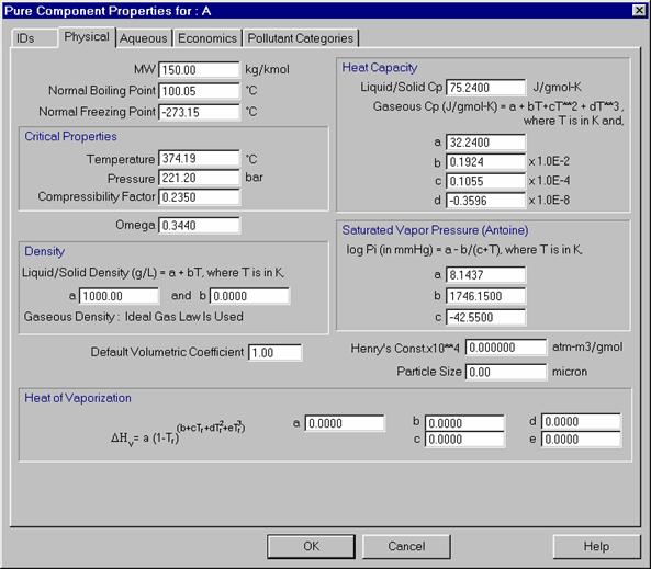
Editing the properties of component A.
The table below summarizes the steps necessary for building flowsheets. The remainder of this section will
describe each of these steps in detail as they are performed during the creation of the example process.
To build a flowsheet:
1. Add processing steps (unit procedures) to the flowsheet. A unit procedure is defined as a series of operations that take place within a piece of equipment. Please note that continuous unit procedures are equivalent to unit operations. To introduce a new procedure, select a unit procedure from the Unit Procedures menu, and click somewhere on the flowsheet to lay down the processing step (see Adding a Unit Procedure in the on-line Help facility for more information). Then add operations, such as Charge, Transfer, React, Extract, etc. to each unit procedure by double-clicking the unit procedure icon (or right-clicking the icon and choosing Add/Remove Operations). Different operations are available to different unit procedures.
Helpful Hint: If you would like to know more about a particular unit procedure, you can look it up using the Help facility. This facility contains a general description of each procedure, links to its operation models, a diagram of the input and output ports, and much more. As a shortcut to the Help for any procedure, you can click the Help icon (the one with a question mark and an arrow on it) and then click on the unit procedure icon you are interested in. Alternatively, you can click on the unit procedure icon to highlight it, and then hit the F1 key.
2. Repeat step (1) for all the unit procedures involved in the current design case. You dont have to add all the procedures at once. You can always add or remove procedures as desired at a later stage of the design. It is recommended that you begin your design with just a few procedures, and add more steps after you have determined that your streams and operations have been initialized correctly, and your mass balances make sense.
3. Introduce connections between the processing steps by drawing all the intermediate streams. To create an intermediate stream, click on an output port of the upstream procedure, continue clicking on intermediate points (if you want to create your own elbows) and finally click on an input port of the destination procedure (see Drawing: Streams in the on-line Help facility for more information).
4. Introduce the input streams and the output streams. To create an input stream, click on the desired starting location, continue clicking on intermediate points if you want to create elbows and finally click on an input port of the target unit procedure. To create an output (product or waste) stream, click on an output port of a unit procedure, continue clicking on intermediate points (if you want to create your own elbows) and finally double-click on the desired ending location.
NOTE
If similar sections of a flowsheet repeat themselves, you can use the copy and paste utility of SuperPro Designer to accelerate the deployment of all processing steps. You can also copy whole sections from one flowsheet to another. Simply open the source flowsheet, select the procedures and streams of the desired section and copy them (select Edit: Copy from the main menu, or click on the copy button of the toolbar). Then open the destination flowsheet, click where you want to have the section laid out, and paste it (select Edit/Paste from the main menu, or click on the paste button.)
To Add a Unit Procedure to the Flowsheet
First select
the desired unit procedure from the Unit
Procedures menu. For our example,
please select Unit Procedures/Vessel
Procedure/in a Reactor. Notice that
after you select this unit procedure, the mouse cursor changes to:
![]()
indicating that your next mouse click on the flowsheet will lay down the
reactor unit procedure icon in that location. Please click near the left side of the flowsheet to place the Vessel
Procedure icon.
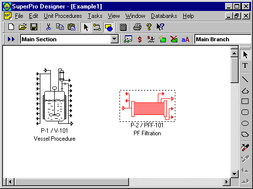
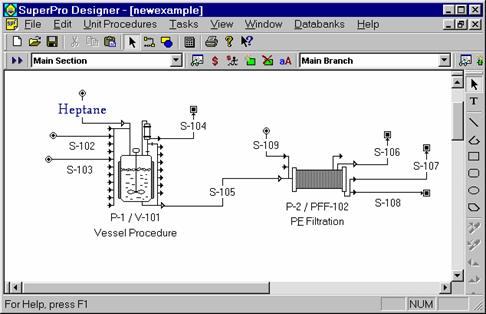
After you have added the Vessel Procedure to the flowsheet, please add a Plate and Frame filtration procedure by selecting Unit Procedures/Filtration/Plate and Frame Filtration, and then clicking somewhere to the right of the Vessel Procedure icon. Your flowsheet should now look something like this:
Note: If you decide to abort the addition of the new unit procedure, you can simply hit the ESC key. If you intend to introduce the same unit procedure several times, you can use the following shortcut: after you have laid down the first unit procedure icon, hold down the Ctrl and Shift keys and click where you want the next copy of the process step to be located.
If You Wish to Move a Unit Procedure
Select the desired unit procedure icon by clicking on it with the mouse. If more than one icon needs to be moved at the same time, you can either group-select them by dragging an enclosing rectangle around them, or you can edit the selected icon set by adding or removing icons one by one. To add an icon to the selection set, click on it while holding down the Ctrl key. Note that if the icon was already in the selection set, it will be de-selected if you Ctrl+Click on it.
Drag the selected icon to the new location. If the selection set has more than one icon, drag any member of the selection set and all icons will move simultaneously. If you want to move the selected set of icons one pixel at a time, you can use the arrow keys.
NOTE: When you move a unit procedure icon, which has streams, attached to it, all streams will move with it. If the destination and source icons of a stream move, then the stream will keep its structure intact and move with them. If one of the streams ends remains anchored while the other end is being moved, then the stream will adjust its first and/or last elbow to accommodate the change of location. Adding and moving stream lines will be explained later in this example.
If You Wish to Delete a Unit Procedure
Select the unit procedure icon you wish to delete by clicking on it with the mouse. If desired, you can delete multiple procedures at once (see To Move a Process Step above to learn how to select multiple unit procedures).
Hit the Delete key or select the Edit/Clear option from the main menu. The selected unit procedure(s) will be erased.
NOTE: When you delete a unit procedure, all streams attached to it will be deleted with it.
If You Wish to Cut/Copy and Paste a Unit Procedure
SuperPro Designer allows you to place a selection of unit procedures and streams onto the clipboard by cutting or copying them and later pasting them into another area of the same flowsheet. In addition, you can use the Cut/Copy and Paste features of the program to copy whole sections from one flowsheet to another. To do this, simply select the desired unit procedure icon(s), and then select Edit/Cut (or Ctrl+X) to cut the icons or Edit/Copy (or Ctrl+C) to copy the icons. Next, paste the unit procedures onto another area of the flowsheet, or onto different flowsheet by selecting Edit/Paste (or Ctrl+V).
NOTES:
You cannot copy and paste streams alone. Streams are placed onto the clipboard only if their source and destination unit procedures (when they exist) are also placed on the clipboard.
When pasting unit procedures from the clipboard onto a flowsheet, you should be aware that certain features of the original unit procedures are not transferred into the newly created copy:
a. Stream connections to any unit procedures not included in the pasted set.
b. If the start time of the first operation of the pasted unit procedure was defined on a relative basis (e.g., with respect to the start or end of another operation in some other procedure), then the scheduling of the pasted procedure is reset to remove the coupling.
c. If the original unit procedure was sharing equipment with another procedure, the pasted procedure is reset to be executed in its own equipment.
Pasting streams and certain processing steps with component-related specifications from one flowsheet to another is not possible unless all components of the source flowsheet exist in the destination flowsheet as well. If that is not the case, the program will automatically expand the set of registered components in the destination flowsheet to include the missing ones.
Adding Streams to the Flowsheet:
After you have placed unit procedures on your flowsheet, you may add stream connections to the icons. There are three types of streams: feed streams, intermediate streams, and product (output) streams. Feed streams do not have a source unit procedure and in batch processing they are mainly utilized by charge operations. Intermediate streams connect two unit procedures, and they are used to transfer material from the source to the destination unit procedure. Product streams do not have a destination unit procedure. All streams are automatically identified with a stream tag.
In order to add streams to the
flowsheet, you much first enter Connect
Mode by clicking on the Connect Mode
button ![]() of the main toolbar. When you do this, the cursor icon changes to
the following:
of the main toolbar. When you do this, the cursor icon changes to
the following: ![]() to indicate that you are in Connect
Mode. Next you can add the feed,
intermediate, and product streams as follows:
to indicate that you are in Connect
Mode. Next you can add the feed,
intermediate, and product streams as follows:
1. Adding a Feed Stream: Click
any unoccupied area on the open screen to initiate drawing of the stream and
then click on the appropriate inlet port of the destination unit procedure to
terminate the stream. Notice that as the
cursor moves over the inlet and outlet ports, it changes to a Port Cursor:
![]()
You must make sure the cursor looks like
this before you click to attach the stream to a port. Otherwise the computer will simply add a
stream elbow at this point and will not actually terminate the stream. If you accidentally miss the stream port, you
can simply hit ESC to cancel the stream-drawing process. Then you can restart the stream-drawing
process by clicking the Connect Mode button again.
Between initiation and termination of the feed stream, the mouse may (optionally) be clicked at intermediate points to create right angle bends; this permits customization of the stream route and flexibility in flowsheet design. SuperPro Designer automatically draws the feed stream symbol and labels the stream.
2. Adding an Intermediate Stream: Click on the appropriate outlet port of the source unit procedure and then on the appropriate inlet port of the destination unit procedure to terminate the stream. Be sure to wait until the Port Cursor icon (explained above) is displayed before attempting to begin or terminate a stream on a port. As before, you can create specific routing by clicking the mouse wherever a right angle bend is desired.
3. Adding a Product Stream: Click on the appropriate outlet port of the source unit procedure and then double-click somewhere to terminate the stream line. When you double-click, the cursor should be close to the last drawn horizontal or vertical line segment. Note that SuperPro Designer automatically draws the product stream symbol.
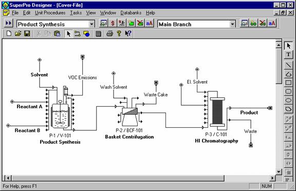
At this point, please add feed, intermediate, and product streams to your example process. Your flowsheet should now look something like this:
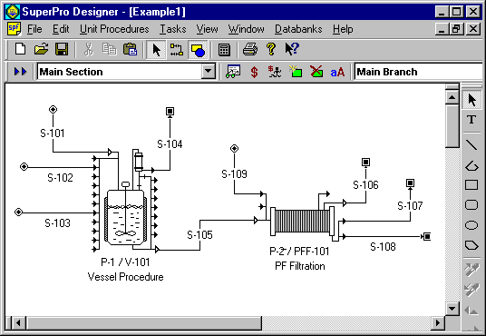
The example flowsheet with streams added.
Notes:
1) Hitting ESC while drawing a stream terminates the stream drawing process. To get back into stream mode after hitting ESC, simply hit the Connect Mode button again.
2) In many unit procedures, there are dedicated ports, such as feed, vent, cake removal, filtrate removal, etc.. To see which ports are dedicated to each function, you can look up the desired unit procedure in the Help menu. As a shortcut to the Help for any procedure, you can click the Help icon (the one with a question mark and an arrow on it) and then click on the unit procedure icon you are interested in. Alternatively, you can click on the unit procedure icon to highlight it, and then hit the F1 key. A portion of the Help for the Plate and Frame Filtration unit procedure appears below. Notice that the dedicated ports are labeled next to the filter icon. The Help facility also contains a general description of each procedure, links to its operation models, and much more.
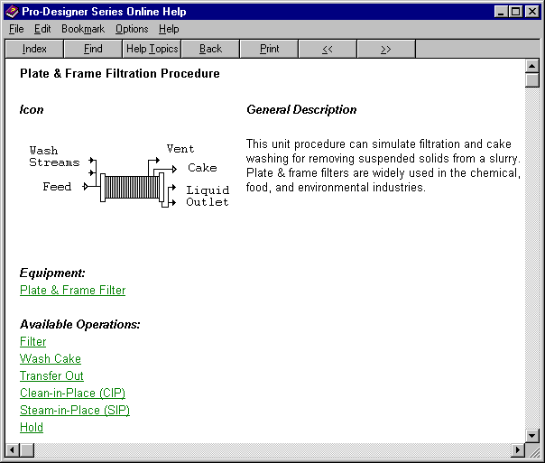
A Portion of the Help file for Plate and Frame Filtration.
When you are finished drawing
streams, you should exit Connect Mode and return to Select Mode. This is done by
hitting ESC or clicking on the toolbar button that looks like: ![]()
|
The stream context menu. |
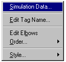
When SuperPro is in Select Mode and the mouse is over a stream line, the arrow will change to indicate the availability of a stream context menu (see figure to the left), which may be activated by clicking the right mouse button. Through this menu you can view and edit (for input streams only) the composition, flowrate, and other stream properties. You may also change the Tag Name (label), adjust the Elbows, and edit the Style (e.g., label and line color, line thickness, etc.) of any stream. Note that double-clicking on a stream line with the left mouse button is equivalent to selecting the Simulation Data menu item. |
At this point, please right-click on the Vessel Procedure input stream S-101 and choose Edit Tag Name. Change the name of this stream to Heptane and click OK. Then right-click the Heptane stream line, select Style/Edit Style, and Click on the Name Tag tab (see below).
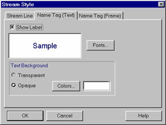
Now click the Fonts button to change the style, size and color of this stream tag name. After clicking OK, your flowsheet should look something like this:
Please see the on-line Help facility for additional information on stream-drawing.
Adding Operations to Unit Procedures:
The first step toward initialization of unit procedures is to add relevant operations to each unit procedure. This can be done by double-clicking a unit procedure icon to bring up the following dialog box:

At this point, please add a charge operation to the Operation Sequence in your Vessel Procedure by double-clicking the word Charge in the list on the left. Alternatively, you can add the operation by highlighting the word Charge and clicking the Add or Insert buttons. Now add two more Charge operations, a React (Stoichiometric) operation, and a Transfer Out operation (so that your dialog box looks like the figure above). Then click OK to return to the flowsheet.
Note: If you make a mistake while adding operations, you can delete the operation by selecting it in the Operation Sequence list and hitting the Delete button. If you add an operation in the wrong order, you can click and drag it to a different position in the Operation Sequence list. To change the name of an operation, select it and hit the Rename button.
After you have added operations to the Vessel Procedure, double-click the Plate and Frame filter icon to add operations to it. Notice that by default, this unit procedure has an operation (Filter-1) assigned to it. Use the same method as before to add a Cake Wash operation and a Transfer Out operation to this unit procedure (in addition to the Filter operation which is already present).
Note: Double clicking on a continuous procedure (e.g., a Centrifugal Pump) that is present in a continuous flowsheet brings up the dialog window of its essential operation instead of the dialog above. In other words, a unit procedure in a continuous flowsheet behaves like a unit operation.
Initializing the Operations:
The next step is to initialize each of the operations that have been added to the unit procedures. To do this, please right-click the mouse over a unit procedure icon to bring up its context menu (see figure below).
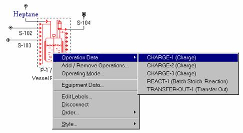
The meaning of each portion of the context menu (above) is explained below:
1) The Operation Data menu allows the user to access and modify the simulation parameters for each operation in this unit procedure. (Note the Operation Data menu will not appear until at least one operation has been added. Furthermore, if only one operation is present in the unit procedure, no drop-down list will appear to the right of the context menu. In this case, simply click on the Operation Data line of the context menu to bring up the parameters for the operation).
2) The Add / Remove Operations menu allows the user to add new operations to the procedure, delete existing ones, rename them, and rearrange their order. This is the same dialog that is brought up when you double-click on a batch unit procedure.
3) Through Operating Mode the user can specify the number of cycles per batch and certain other scheduling related parameters.
4) Through Equipment Data the user can select the equipment sizing mode (Design or Rating) and specify size and purchase cost parameters.
5) Through Edit Labels the user can change the name of the procedure (e.g., P-1 in the above procedure), the name of the equipment (V-101 in the above case), and the description of the procedure (Vessel Procedure in the above case).
6) The Disconnect option allows the user to disconnect a unit procedure from all stream lines. If you need to reverse the flow of material through the icon (by default the material flow through any icon is from left to right) you can also flip the icon horizontally. To flip an icon horizontally, select the Flip (reverse flow direction) option from the context menu. Note that the Flip icon option is only available when the unit procedure is not connected to other steps via material streams. You can also flip the icon by selecting it and clicking on the Flip Horizontal button of the Visual Object Toolbar.
7) The Order option of the context menu allows you to force the unit procedure icon to appear behind or in front of other icons, text, etc.
8) The Style option allows you to edit such things as the icon color, the name tag color and font, etc.
At this point, please select Operation Data: Charge-1 from the vessel procedure context menu (as was done in the figure above). This will bring up the following dialog:
The Operation Data dialog for the first Charge operation in the Vessel Procedure.
The Operation Data dialog allows you to specify the operating conditions, emissions data, labor, scheduling, etc. for each operation. Different tabs of input fields are available for different operations. To initialize the Operating Conditions tab for the first charge operation in this example, you will first need to specify where the material being charged is coming from. To do this, use the drop-down menu at the top of the Operation Data dialog box to select the stream which you renamed Heptane earlier in this chapter. Then click the Edit Amount button to access the stream data for this stream (see figure below). To add heptane to the stream, double-click its name in the Registered Ingredients list on the left side of the dialog box. Then specify the amount to be 800 kg/batch by clicking in the Flowrate (kg/batch) box and typing 800.

The Heptane stream dialog.
Notes:
You can charge multiple components in the same stream if you wish. To do this, simply add additional component names from the Registered Ingredients (Pure Components or Stock Mixtures) list and specify their amounts. The computer will automatically calculate the mass % and concentration (g/L or mole/L) of each ingredient, the streams density (if it is not set by the user), the volumetric flowrate and the activity of the stream. Alternatively, you can click on Ingredient % and specify the total mass or volume flow and the mass % of each component. If you prefer to specify and view flowrates on a molar basis, just click on View Molar Flow on the bottom of the dialog.
As an alternative to going through the Operation Data dialogs to edit stream properties, you can initialize and edit input streams directly from the flowsheet itself. To do this, open the stream context menu by clicking the right mouse button over a stream line and selecting Simulation Data. This will bring up the same dialog box as the one shown above. You could also double-click the left mouse button on a stream line to generate this dialog box. Note that only the feed streams to the flowsheet need to be specified. The flowrates and compositions of intermediate and output streams are calculated by the program. However, the user can specify the density and volumetric contribution coefficients of such streams.
Some operations (e.g., cake wash, column elution, etc.) that utilize input streams automatically calculate the amount of material that they require. In such cases the user only needs to specify the composition of an input stream; its total flow can have any positive value.
In addition to pure components, mixtures can be fed (or charged) into a process step using an input stream.
For biotech processes, the extracellular percentage (Extra-Cell %) of an ingredient represents its fraction that is in the bulk solution (as opposed to inside the cell). For more information on this topic, please refer to the b-Galactosidase example in Chapter 3.
If the operating mode of a flowsheet is batch, all flowrates are reported on a per batch basis (or per cycle of source or destination process step). If the plant is set in continuous mode, then all flowrates are reported on a per hour basis. The choice for mass units can be made from each streams dialog. This choice overwrites the default choice made by the specification at the Edit: Flowsheet Options: Preferences: Stream Report Options dialog.
The Env.Properties tab of a stream dialog displays the concentrations and daily throughputs of the environmental and aqueous properties of the stream (TOC, CaCO3, TP, TKN, COD, ThOD, BOD5, BODu, etc.) All values are for display only and cannot be edited by the user through this dialog box. However, the environmental properties of the pure components (that contribute to the above stream properties) can be edited through the Tasks: Register Components & Mixtures : Pure Components dialog.
For more information on stream properties, please refer to the Help facility.
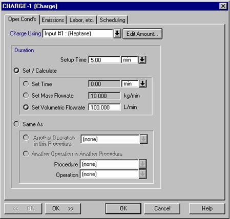
After you have specified the charge amount of Heptane, click OK to return to the Operation Data dialog for Charge-1. Notice that there are several ways that the duration of this operation can be specified. For this example, change the setup time of your charge to 5 minutes and set the Volumetric Flowrate to 100 L/min. Please also visit the Emissions, Labor etc, and Scheduling tabs to see what fields they contain. A brief description of each of these tabs follows:
Emissions tab: Here the user can specify which volatile organic compounds (VOCs) will be emitted, whether a sweep gas will be used (for emissions associated with reaction and crystallization operations), and what temperature the vent condenser should be set at. SuperPro is equipped with VOC emission models that are accepted by EPA. Please consult the on-line Help Facility for more information on emission calculation models. For the heptane charge in your example process, please click in the Perform Emission Calculations box. Then Click in the Emitted box next to the Heptane component. After the simulation, please remember to visit the dialog of stream S-104 and check the amount of emitted Heptane. For particulate and other components for which emission models are not available, the user can specify the Emission %.
Labor tab: Here the user can specify labor requirements and auxiliary utilities.
Scheduling tab: The right-most tab of a batch unit procedure is always the Scheduling tab. Through this tab, the user specifies the start time of an operation relative to the start or end of other operations in the same or different procedures. For unit procedures in continuous mode, no scheduling information is required.
Note: Depending on the complexity of an operation, additional tabs may be employed to display other pertinent variables.

The Emissions tab for the heptane charge.
For this operation, leave all the default values for the Labor etc and Scheduling tabs. Next, click the OK >> button on the Operation Data dialog to move to the second charge operation in this unit procedure. For this operation, use stream S-102 to add 50 kg of material A to the reactor. Also specify a 5 minute setup time and a 20 kg/min charge rate. Leave the default values for the other tabs. Then click the OK >> button to move to the final charge operation. Initialize this the same way as before, but use stream S-103 to add 40 kg of material B. Also change the setup time to 5 minutes and the charge rate to 20 kg/min. Once again, click the OK >> button to move to the next operation (the Batch Stoichiometric Reaction). Notice that the Operating Conditions tab is different for this operation than it was for the Charges, and that several other tabs (Volumes, and Reactions) are present in the Operation Data dialog (more detailed information on reaction operations can be found in the second example that deals with a Synthetic Pharmaceutical process). Starting with the Operating Conditions tab, change the Final Temp to 50 C, the Heat Transfer Agent to Steam, and the Process Time to 6 hours. Leave all the other default values on this tab as they are. Next, referring to the Volumes tab, notice that you can specify a maximum and minimum working to vessel volume ratio. Change the Max Allowable working/vessel volume to 80%. Then move to the Reactions tab (see figure below).
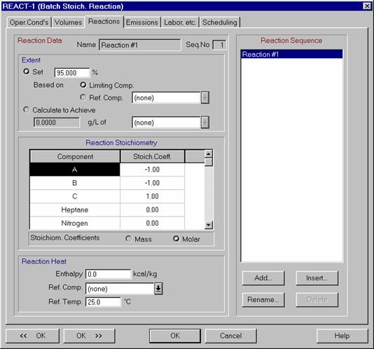
The Reactions tab of the Batch Stoichiometric Reaction Operation.
In this tab, you will need to specify the parameters describing a reaction in which 1 molecule of reagent (A) combines with 1 molecule of reagent (B) to form each molecule of product (C):
A + B à C
For this example, the molar stoichiometric coefficients would be -1, -1, and 1, respectively, for A, B, and C. For more information on specifying reaction coefficients, please see the synthetic pharmaceutical intermediate example in Chapter 4. In addition to specifying the stoichiometric coefficients, you will need to specify the extent of reaction. For your example, set the Extent to 95%, as was done in the figure above. Next, click the OK >> button to move to the Transfer Out operation (leave all the default values for the Emissions, Labor etc, and Scheduling tabs.)
In the Transfer Out dialog, use the drop-down menus at the top of the screen to specify which stream line will be used for the transfer operation, and what the destination unit procedure will be (see below). In addition, in order to accurately capture the time required for this operation, set the duration to be the same as the filtration duration in P-2. This will ensure that the reactor will still be considered utilized during the filtration, since the reactor will not be completely emptied until the filtration is complete. You can leave the default values for the other tabs in this dialog.

The Transfer Out operation dialog.
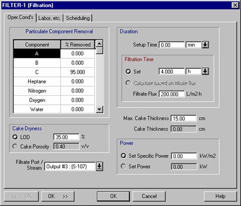
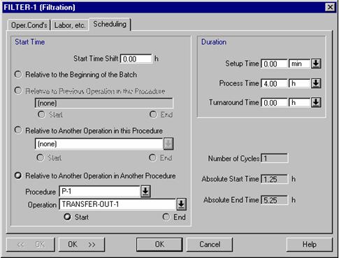
Next you will need to initialize the operations in the Plate and Frame Filtration unit procedure. To do this, right-click on the filtration procedure and choose Operation Data: Filter-1. For this example, assume that components A and B are completely soluble in Heptane, and component C is virtually insoluble. Therefore, in the Particulate Component Removal section of this dialog box, please specify that 95% of your product C will remain on your filter, but the other components will not be preferentially retained (everything else has 0% removed). Also notice that you can specify a Cake Dryness based on LOD (loss on drying) or Cake Porosity. Please change the LOD for your filtration to 35%. This value will cause a portion of the Heptane (and any soluble components) to be held in your wet cake. By specifying a LOD of 35%, you are telling the program that only 65% of the wet cake is the insoluble product C. Next, please visit the Scheduling tab of the filtration operation. By default, the first operation in any batch unit procedure is scheduled to start relative to the beginning of the batch. In order to accurately schedule your filtration, you will need to change the Start Time to be relative to the start of the Transfer Out operation in procedure P-1.
The Filtration operation dialog.
The Scheduling tab of the Filtration operation.
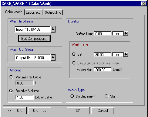
Next, click OK >> to move to the Cake Wash operation (see figure below). Here you will need to specify which stream will provide the wash solvent and which one will remove the waste (S-109 and S-108 in this case). In addition, you will need to specify what solvent is used for the wash. To do this, press the Edit Composition button and select Heptane. You will also need to enter a value for the amount of Heptane used (although the program will override this value later during simulation). Then click OK to return to the Cake Wash dialog. Notice that from this dialog you can specify the volume of wash to use, based on the cake volume or a set value. Please keep the wash amount as 1 L/L of cake, use a wash time of 30 minutes, and change the wash type to slurry from displacement. A slurry wash will essentially dilute the soluble components trapped in the cake and remove most of them in the wash stream, whereas a displacement wash will remove the soluble components from the cake in a plug-flow fashion.
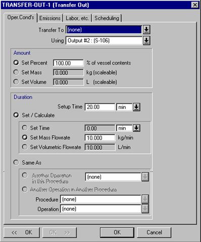
Finally, click the OK >> button to initialize the Transfer Out operation in this unit procedure (see figure below). In this operation, you will need to specify that you are going to transfer out the cake using a specific stream (S-106 is the only one available in this case) and the transfer will take a certain amount of time (10 kg/min in this case). Then Press OK.
You have now finished initializing the operations and streams for this example flowsheet.
At this
point, you can use the Tasks: Solve
M&E Balances
option from the main menu to perform the simulation. This will cause the program to perform the
mass and energy balances for the entire flowsheet, estimate the sizes of all
pieces of equipment in Design Mode, and model the scheduling of each piece of
equipment. As a short-cut for performing simulations, you may hit Ctrl+3 or simply click on the following toolbar button: ![]()
The simulation results can be viewed in the following ways:
1.) The calculated output variables for each operation can be viewed by revisiting the corresponding Operation Data dialog windows (right-click on the desired Unit Procedure icon, then choose the operation you are interested in). For instance, you can see how long each of the Charge operations takes (recall that their durations were based on a given mass to be charged and a flowrate).
2.) The calculated flowrates and compositions of intermediate and output streams can be viewed by revisiting the Simulation Data dialog windows of each stream (double-click on any stream line to see its Simulation Data dialog).
3.) A report containing information on raw material requirements, stream compositions and flow rates, as well as an overall material balance, can be generated by selecting the Tasks: Generate Stream Report (SR) option from the main menu. The resulting report can be viewed by selecting the View: Stream Report option of the main menu. This report has tables that include an overview of the process, a listing of the raw material requirements, a listing of the compositions of each stream, and an overall component balance. Please generate and view the Stream Report now.
4) To see the calculated equipment sizes, right-click on a unit procedure icon and choose the Equipment Data option. The figure below displays the Equipment Data for the Plate & Frame filter in this flowsheet. Through this tab, you can provide information for equipment sizing, selection, and purchase cost estimation (the cost estimation features will be explained in greater detail later in this chapter). All unit procedures have two options for equipment sizing: Design and Rating. By default, all equipment starts in Design Mode. In this mode, SuperPro will determine the required equipment sizes based on operating conditions and performance requirements. Usually, there are physical limitations on the available size of processing equipment. For example, a Plate & Frame filter may not be available with a volume greater than 80 m2. When you are in Design Mode, you must specify the maximum available size for the equipment involved. If the calculated equipment size exceeds the maximum allowable size, SuperPro will employ multiple pieces of equipment (sized equally) with sizes that do not violate the maximum available size. For your example flowsheet, a filter size of roughly 1.46 m2 should have been calculated. This number was calculated from the volume of material that is processed per cycle, the filtrate flux, and the filtration time.

The Equipment Data tab of the Plate & Frame Filter.
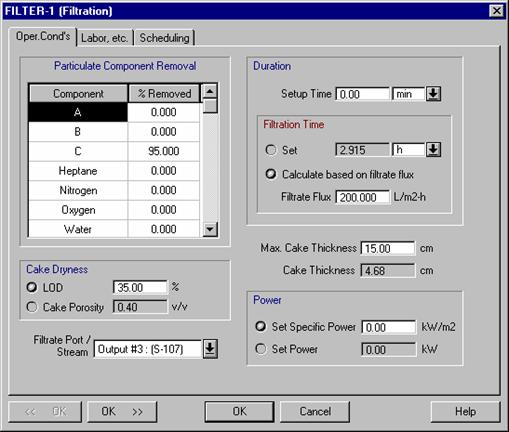
If you change the equipment sizing method to Rating Mode, you can specify the size and number of units. SuperPro will then take this information into account in the simulation calculations (equipment size and number of units may affect the material and energy balances, the process time, etc.). Switching to Rating Mode may also affect the interface of some operations of that procedure. To experience this, please change the size of the filter to 2 m2 and revisit the dialog of the filtration operation (see figure below). In this case, you need to specify either the filtration time or the average filtration flux (in Design Mode, you need to specify both). Please set the filtrate flux to 200 L/m2 hr and redo the calculations to determine the new filtration time. In general, most batch operations have the capability of calculating their cycle time when the equipment size is specified (Rating Mode). Through the equipment tab, you can also select the specific piece of equipment that is going to carry out the processing step. By default it is assumed that each unit procedure is carried out in its own (exclusive) equipment. However, two (or more) different procedures can share equipment if they are in batch operating mode and the entire flowsheet is also in batch mode. For more information on equipment sharing, please consult the on-line Help Facility (search for Equipment Sharing).
At this point you have completed the basic initialization steps for the streams, operations, and equipment. As you become more familiar with SuperPro Designer, it will take much less time to do these activities. For instance, all the steps that we have done thus far in this example could be performed in about 15 minutes if you were already familiar with how to use SuperPro.
Important note about building and initializing large flowsheets when you design complex flowsheets, keep in mind that you dont have to add all the unit procedures at once. You can always add or remove procedures as desired at a later stage of the design. For complex flowsheets, it is highly recommended that you begin your design with just a few unit procedures and add more of them only after you have simulated the first unit procedures and determined that the streams and operations have been initialized correctly and your mass balances make sense.
If you have specified the entire plants mode of operation as batch, which is the case for your example flowsheet, you should provide process scheduling information before performing a simulation. SuperPro Designer allows you to specify the following scheduling data:
|
For each operation: a. the process time, b. the setup and turnaround times, c. the starting time, and d. the number of cycles (at the procedure level). |
. For the entire plant: e. the annual operating time, f. the number of campaigns per year, and either: g1. the number of batches per year, or g2. the effective batch time, or g3. the effective batch time slack. |
Scheduling of individual operations was explained in Chapter 2.5.5. Each operation scheduling dialog allows you to specify the starting time of the operation relative to the beginning of each batch or relative to the start or end of other operations in the same or different procedures. You may also specify the process time (if it is not calculated by the model), the setup time, and turnaround time.
To specify the number of cycles per batch of a procedure (and all operations within that procedure), simply right-click on the unit procedures icon and choose Operating Mode. By default, all procedures start with one cycle.
To specify scheduling for an entire plant, select Tasks: Recipe Scheduling Information (see figure below).
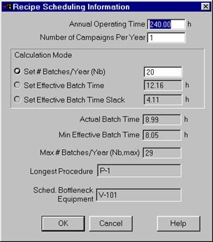
For your example process, please change the Set # Batches/Year field to 20. This implies that your example process will be run in a pilot plant 20 times this year (it is assumed that the equipment used by this process is used by other processes the rest of the year.) In addition, please change the annual operating time for this process to 240 hours to reflect the completion of one batch during every 12-hour shift.
Based on the scheduling information and the annual operating time specified for the plant, the system will do the following:
1. Make sure there is no conflict created by the specified start time and end time of processing steps. Conflicts can be created if the cycle times of procedures that share equipment overlap.
2. Make sure there is no conflict between the specification of annual operating time, the number of batches, and the effective plant batch time (as calculated from all the procedures).
3. Calculate the plants batch time, the plants effective batch time, the plants minimum effective plant time (with maximum batch overlapping), the maximum number of batches possible, the longest procedure (i.e., the procedure with the longest total cycle time) and the scheduling bottlenecking equipment (the equipment with the longest occupancy time).
A variety of
scheduling, equipment utilization and resource tracking tools are included in
SuperPro Designer. These include
Operations and Equipment Gantt Charts,
Please generate the Operations Gantt Chart for your example process by selecting Tasks: Gantt Charts: Operations GC from the main menu. It should look similar to the figure below. The left view (spreadsheet view) displays the name, duration, start time and end time for each activity whose bar line is shown straight across on the chart (all information is presented for viewing purposes only). You can use the left view to expand and/or collapse activity summaries by clicking on the + or rectangle showing at the left of the name of the activity. The right view (chart view) displays a bar for each activity participating in the overall scheduling and execution of the recipe.
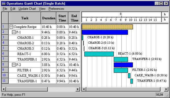
From the Gantt Chart interfaces you can modify the scheduling parameters of each procedure and operation as well as the scheduling parameters for the entire plant (i.e., annual operating time, number of batches per year, etc.). In fact, anything you can accomplish with the scheduling interfaces described earlier in this chapter, you can also accomplish from the Gantt chart interface. In order to edit scheduling parameters from this interface, simply right-click on the bar of the procedure or operation which you are interested in. This will bring up the Operating Mode dialog (in the case of procedures) or the Operation Data dialog (in the case of operations.) To view and edit the scheduling information for the entire batch, right-click on the bar which corresponds to the Complete Recipe (at the top of the chart) and choose Recipe Scheduling Info. After you have edited a scheduling parameter, you must click the Update Chart button on the Gantt Chart main menu to see the changes. As you can see, these Gantt Charts present you with a graphical way to set the scheduling parameters of each processing step and immediately visualize the effects on the entire batch production. Please refer to the examples in Chapters 3 and 4 to see Gantt Charts for more complex processes.
Another way of visualizing the execution of a batch process as a function of time is by selecting View : Equipment Utilization Chart. The figure below displays the Equipment Utilization Chart for three consecutive batches of the process of this example. White space represents idle time. The equipment with the least idle time between consecutive batches is the time (or scheduling) bottleneck (V-101 in this case) that determines the maximum number of batches per year. Its occupancy time (9.44 hours in this case) is the minimum possible time between consecutive batches (also known as Min. Effective Plant Batch Time). The actual time between consecutive batches (also known as Effective Plant Batch Time) is 12 hours. The plant batch time (the time required to complete a single batch) is 10.4 hours.
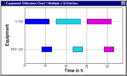
SuperPro also generates utilization charts for auxiliary equipment, such as clean-in-place (CIP) and steam-in-place (SIP) skids.
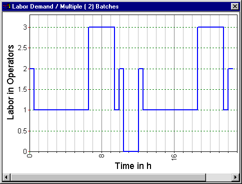
In addition to creating Gantt charts for equipment utilization and operations, SuperPro Designer automatically generates graphs of resource demand as a function of time for such things as heating and cooling utilities, power, labor, and raw materials. To view these graphs, select View: Resource Chart, and then choose the desired resource from the drop-down menu. The figure below displays the labor requirement resource demand graph for two consecutive batches. As you can see, three operators are required to handle this process.
SuperPro is equipped with powerful throughput analysis and debottlenecking capabilities. The objective of these features is to allow the user to quickly and easily analyze the capacity and time utilization of each piece of equipment, and to identify opportunities for increasing throughput with the minimum possible capital investment. For a detailed throughput analysis example (based on the process of the second example), please see Chapter 6 or search for Debottlenecking in the Help Facility.
SuperPro performs thorough cost analysis and economic evaluation calculations and generates two pertinent reports. The key initialization steps are described below.
This step must precede economic evaluation, through analysis, and environmental impact assessment calculations. To supply this data, first select the Tasks: Revenue, Raw Material and Waste Streams item from the main menu. You will be presented with a dialog window (see below) where you can classify all input and output streams as raw materials, revenues or wastes (solid, liquid or gaseous) and supply any cost data associated with the classification. By default, the system estimates a purchase or selling price for a stream based on the price of each component and the composition of the stream. The price of a pure component or stock mixture is part of its Properties, which can be edited when Registering Components as described earlier in this chapter. In your example process, please classify all of the output streams (as was done in the figure below). Notice that the Selling Price of the Revenue stream is calculated automatically, based on the streams composition (recall that there is still heptane and small amounts of impurities in our product cake, so the price per kg of cake is less than the $200/kg price of pure component C.) Next, click on the Set By User boxes next to the two liquid waste streams and type in $0.10/kg for the Disposal Cost of each. Finally, select your revenue stream (S-106 below) from the Main Revenue Rate drop-down list, and specify that the unit cost for this process will be reported based on the Component Flow of product C (see below).
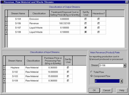
Note: Classification of a stream as a solid, liquid or gaseous waste will cause it to be reported in dedicated sections of the Environmental Impact Report, where a detailed bookkeeping is kept on all chemicals that end up in each waste category. The environmental impact report allows you to evaluate the burden of the process on the environment. Such an assessment assists the designer to focus his/her attention on the most troublesome streams and the processing steps that generate them. A related report, the Emissions Report provides information on emissions of volatile organic compounds (VOCs) and other regulated compounds.
Economic Parameters at the Unit Procedure Level:
All unit procedures have two common dialog tabs through which the user can provide information that affects the capital investment and certain items of the operating cost of that particular step:
1. Information about equipment purchase costs and various adjustments can be provided through the Purchase Cost and Adjustments tabs of the Equipment Data dialog (right click on the vessel procedure and select Equipment Data). By default SuperPro uses a built-in model to estimate purchase costs for each piece of equipment. However, you can override this estimate by either using your own model (click on User-Defined Model) or specifying an exact purchase cost (from a vendor quote, for instance.)
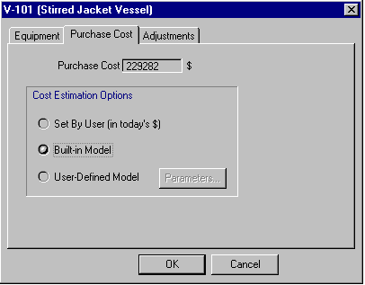
The Purchase Cost tab of the Equipment Data dialog box
Now please click on the Adjustments tab of this dialog to view the % depreciated, material factor, # of standby units, etc. for the reactor. The fields on this tab are described in detail below:
Already Depreciated Portion:
Oftentimes, a piece of equipment has already been either fully or partially depreciated. This can be captured using this variable. Any values other than 0.0% reduce the cost of depreciation but have no impact on the maintenance cost because that cost depends on the full purchase cost and not just the undepreciated portion.
Installation Cost:
This factor is used to estimate the installation cost for each piece of equipment.
Material Factor:
The purchase cost that is estimated using the built-in model corresponds to a certain material of construction that is displayed on this tab. Selecting a different material of construction will affect the equipment purchase cost. Note the material cost factors for each type of equipment can be edited by choosing Databanks: Construction Materials from the menu bar. Additional materials can also be added to the database if you click the Add Material button on this interface. Note a pink -1 in a material factor field represents a lack of data for that combination of material and equipment type.
Standby Units:
For pieces of equipment that are critical to the operation of a process, you may choose to have one or more standby units (in case the regularly used pieces of equipment go down for scheduled or unscheduled maintenance). The number of standby units affects the capital investment but has no impact on maintenance and labor cost.
2. Information about labor requirements can be provided through the Labor, etc. tab of an operations dialog, which is accessed by right-clicking on the procedures icon, and then choosing the desired operation from the Operation Data list. Labor costs can be calculated from either a user-specified overall estimate of the number of labor hours required per year, or from an itemized estimate based on the number of labor hours needed for each individual operation in each unit procedure. Through the same dialog you can specify auxiliary utilities, which have no impact on material and energy balance calculations (they do not affect output stream temperatures). They are only considered in costing and economic evaluation calculations. Auxiliary utilities offer a convenient way to associate utility consumption with generic boxes and other operations that do not calculate utility demand.
Notes:
1) For certain operations, an additional tab of the Operation Data dialog is available for specifying the cost of consumables (in the case of membrane filtration, chromatography operations, etc.).
2) If a piece of equipment is shared by multiple unit procedures, its purchase-cost-dependent expenses (e.g., depreciation, maintenance, etc.) are distributed to its hosting steps based on the occupation time of each step.
SuperPro uses a factor-based method to estimate the capital investment associated with each section of a flowsheet. These factors have been assigned default values that should be reasonable for most cases. However, you should still check these factors to ensure that they are accurate for your situation. You can then adjust the factors to better suit your particular design case. The figure below shows the dialog box that allows you to edit factors used to estimate the direct fixed capital (DFC) of a section. This dialog box is brought up by selecting the appropriate section (Main Section in this case) from the Section drop-down menu, and then clicking on the Capital Cost Adjustments button of the section toolbar (the button with the large dollar sign on it). This dialog box could also be accessed by right-clicking on a blank area of the flowsheet and selecting Section (section name): Capital Cost Adjustments.
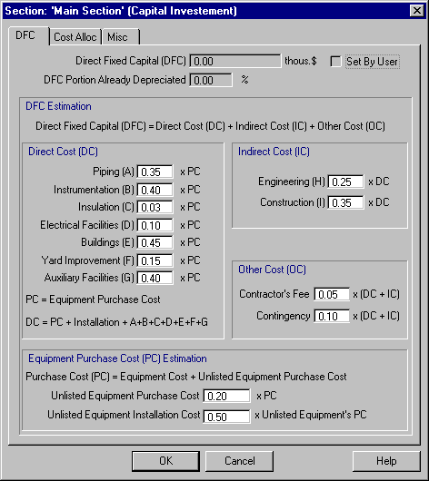
The dialog box for Capital Cost Adjustments.
If an entire section or certain equipment items of a section are utilized by multiple projects (this is quite common for batch processes), the user can specify either the fraction of DFC or the equipment purchase cost that should be allocated to the present project through the Cost Allocation tab of the above dialog.
Through the Miscellaneous tab of the Capital Cost Adjustments dialog, you can adjust parameters that affect the calculation of the Working Capital, Startup and Validation Cost, Up Front R&D, and Royalties.
SuperPro Designer calculates and reports nine cost items for each flowsheet section: Raw Materials, Labor-Dependent, Equipment-Dependent, Laboratory/QC/QA, Consumables, Waste Treatment/Disposal, Utilities, Transportation, and Miscellaneous. The figure below displays the parameters and options available for calculating the equipment-dependent portion of the operating cost. This dialog is brought up by selecting the appropriate section (Main Section in this case) from the Section drop-down menu and then clicking on the Operating Cost Adjustments button of the section toolbar (the button with the small dollar sign and the runner). This dialog box could also be accessed by right-clicking on a blank area of the flowsheet and selecting Section (section name): Operating Cost Adjustments.

Through the Operating Cost Adjustments interface, the user can adjust parameters that affect the Equipment, Labor, Lab/QC/QA, Utilities, and Miscellaneous costs of a section. For your example process, please change the Equipment Cost to be based on an Equipment Gross Rate of $100/hr. This will account for depreciation, maintenance, and miscellaneous equipment expenses.
Next, please visit the other tabs on the above dialog to familiarize yourself with their functions. Notice that in the Labor tab there are various options for specifying the labor costs of your process, including lumped or itemized estimates for both the number of hours required and the labor rate. Furthermore, the Lab/QC/QA tab of the above dialog allows you to specify information for detailed calculation of laboratory, quality control, and quality assurance expenses.
Finally, there are parameters at the flowsheet level that affect the results of project economic evaluation. Through the dialog shown below, for instance, the user can specify various time parameters as well as the interest levels for calculating the net present value (NPV) of the project. This dialog box is brought up by selecting the Edit: Flowsheet Options: Economic Evaluation Parameters option from the main menu. It can also be brought up by right-clicking on a blank area of the flowsheet and selecting the Economic Evaluation Parameters option.
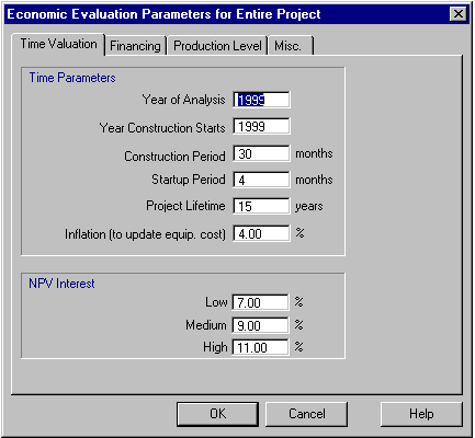
Through the Financing tab of the above dialog, the user can provide information on the financing of the project (e.g., equity versus borrowed money for DFC, working capital, etc.), the method of depreciation, the depreciation period, the salvage value, and the DFC outlay (the spending of direct fixed capital as a function of time).
Through the Production Level tab of the above dialog, the user can specify the capacity utilization profile (production level) for the expected lifetime of the project and provide information for product failure rate and disposal cost of scrapped product.
Through the Miscellaneous tab of the above dialog, the user can provide information for estimation of income tax, advertising and selling expenses, and running royalties.
After simulating the process, you can carry out the economic calculations by selecting Tasks: Perform Economic Calculations. Depending on your interest, you may then do the following:
1.) View the equipment purchase cost for each process step by right-clicking the equipment icon, and then selecting the Purchase Cost tab of the Equipment Data dialog. Remember that the displayed purchase cost is for a single piece of equipment. If the requirements to carry out the specific processing task are such that more than one equipment item (of the same size) is needed, the total cost is the indicated cost times the number of equipment items.
2.) Select View: Executive Summary to view the essential economic evaluation results for the whole process. Please view the Executive Summary of your example process now. It should look similar to the figure below.

3). To view the detailed results which were used to produce the Executive Summary, you will need to generate the Economic Evaluation Report (EER). To generate this report, select Tasks: Generate Economic Evaluation Report. To view it, select View: Economic Evaluation Report. Like the stream report, the EER is a text file which may be read by a variety of text editors and word processors. The same report (like any other report) can also be generated in spreadsheet format by selecting File: Export Reports to Excel. The EER contains tables which give an overview of the process costs, a listing of the cost of each piece of equipment, a breakdown of the fixed capital estimate, summaries of labor, raw material, consumable, waste treatment, and utility costs, a summary of the annual operating cost, a profitability analysis and cash flow analysis, loan information, and breakdowns of the capital outlay and loan payments. You can use the EER to make informed decisions about where to focus resources in the optimization of your process. It can also be used to perform realistic comparisons between various process scenarios (e.g. what-if scenarios and sensitivity analyses). Please generate and view the Economic Evaluation Report now.
4.) Another useful economic report is the Itemized Cost Report (ICR). This report breaks down the costs per flowsheet section. For more information on the contents of the economic reports, please read through the examples in Chapter 3, 4, and 5 or consult the on-line Help.
The demo version of SuperPro Designer comes with a number of case studies in the EXAMPLES subdirectory. The case studies cover chemical, biochemical, and food manufacturing as well as water purification, wastewater treatment and other environmental applications. Before you attempt to create your own design cases, make sure that you spend some time going through the examples. A brief description of the various examples is provided in the table that follows.
Three of the examples in the table below are explained in detail in Chapters 3, 4, and 5 of this manual. Chapter 3 describes the production of the intracellular enzyme b-galactosidase, and is recommended for users in the biotech and food industries. Chapter 4 describes a synthetic pharmaceutical process, and it is recommended for users in the pharmaceutical and specialty chemical industries. Chapter 5 describes an industrial wastewater treatment plant, and it is recommended for users that target water purification, wastewater treatment, and environmental engineering applications.
Description of examples supplied with SuperPro Designer
|
Subdirectory |
Description |
|
AIRCONTR |
This example analyzes a three-step process for removing dust particles and acetone (a VOC molecule) from an air stream. It is recommended for users with interests in air pollution control processes. |
|
BGAL |
This example analyzes the production of b-galactosidase using recombinant E. coli. A detailed description of this follows in Chapter 3. It is recommended for users with interests in biochemical processing. |
|
CHEESE | |
|
CITRACID | |
|
GE |
This example analyzes an effort to minimize generation of hazardous sludge and waste water at a manufacturing facility of General Electric. It is recommended for users with interests in waste minimization, water recycling, and pollution control. |
|
INCINRTR |
This example describes a simple process (a single unit) for analyzing the combustion of sludge in an incinerator. It is recommended for users with interests in incineration and pollution control. |
|
INDWATER |
This example models a simplified version of an industrial wastewater treatment plant. It demonstrates how to track the fate of multiple components (constituents) in a treatment plant. It is recommended for users with interests in industrial and municipal wastewater treatment. |
|
MAMMCELL |
This example analyzes the production of a therapeutic monoclonal antibody using animal cell culture. It is recommended for users with interests in animal cell culture and high value biopharmaceuticals. |
|
MUNWATER |
This example focuses on the modeling and retrofit design of a municipal wastewater treatment plant. It consists of three design cases. The first, mwwt4_0a.spf , represents a typical activated sludge plant without any process steps for nitrogen removal. The second, mwtw4_0b.spf, represents a modified Ludzack-Ettinger process for nitrogen removal. The third, mwtw4_0c.spf, represents a 4-stage Bardenpho process for nitrogen removal. It is recommended for users with interests in industrial and municipal wastewater treatment. |
|
SYNPHARM |
This example analyzes the production of a synthetic pharmaceutical intermediate, which is formed by condensation of quinaldine and hydroquinone. Several reaction and separation steps are involved in the synthesis and purification of the product. A detailed description of this process is included in Chapter 4 of this manual. This example is recommended for users with interests in manufacturing of synthetic pharmaceuticals and specialty chemicals. |
|
UPWATER |
This example deals with water purification (for producing ultrapure water) and wastewater treatment at a Semiconductor Manufacturing Facility. Evaluation of recycling options for minimizing city water use and waste water disposal are included. |
This chapter briefly describes how to use the demonstration program to develop and analyze a flowsheet for the production of b-galactosidase, an intracellular enzyme produced by E.coli. A more detailed description of this process can be found in EXAMPLESBGAL BGAL.DOC. Furthermore, the SuperPro flowsheet for this example can be loaded by double-clicking the BGal4_0b.SPF file within the BGal folder. Alternatively, if you already have SuperPro running, you can select the File: Open option from SuperPro Designers main menu. Then find the file named BGal4_0b in the ExamplesBGal folder, select it, and click OK. We suggest that you keep the design case flowsheet window open as you read the remainder of Chapter 3. However, you should not edit the flowsheet file until after you have finished reading through this chapter.
The figure on the next page shows the entire flowsheet for the b-Galactosidase process (for a better quality printout of this figure, please use the printing capabilities of SuperPro).
b-Galactosidase is mainly used in the utilization of cheese whey. More specifically, immobilized reactors with b-Gal have been developed to convert lactose found in cheese whey to glucose and galactose, yielding a sweetened product which can be used as an additive to ice cream, egg-nog, yogurt, and other dairy products. Another application of b-Gal is in the treatment of milk products. A significant number of people are lactose intolerant and cannot digest milk or milk products. Production of lactose-free milk products (using b-Gal reactors) allows those people to digest them.
The b-Galactosidase enzyme is normally produced by E. coli up to 1-2% of total cell protein under conditions of induction of the lac operon. Using genetic engineering, the level can go up to 20-25% of total protein. In this example, an easily attainable level of 10% is assumed.
This example analyzes a plant that produces 11,500 kg of b-Gal per year in 134 batches. Several files have been included with this example:
BGal-a: This file represents the process at an early stage of plant design. All equipment is in Design Mode, meaning that all equipment sizes and throughputs are calculated as opposed to being specified by the user.
BGal-b: This file shows the plant after equipment sizes have been specified for key pieces of equipment. In addition, some equipment is reused for multiple unit procedures. The BGal-b file was used to produce the tables and graphs in the rest of Chapter 2.3.
BGal-c: This file is the same as BGal-b, except that final product formulation and packaging unit procedures have been added.
We will focus on the BGal-b file for the rest of our process
description.
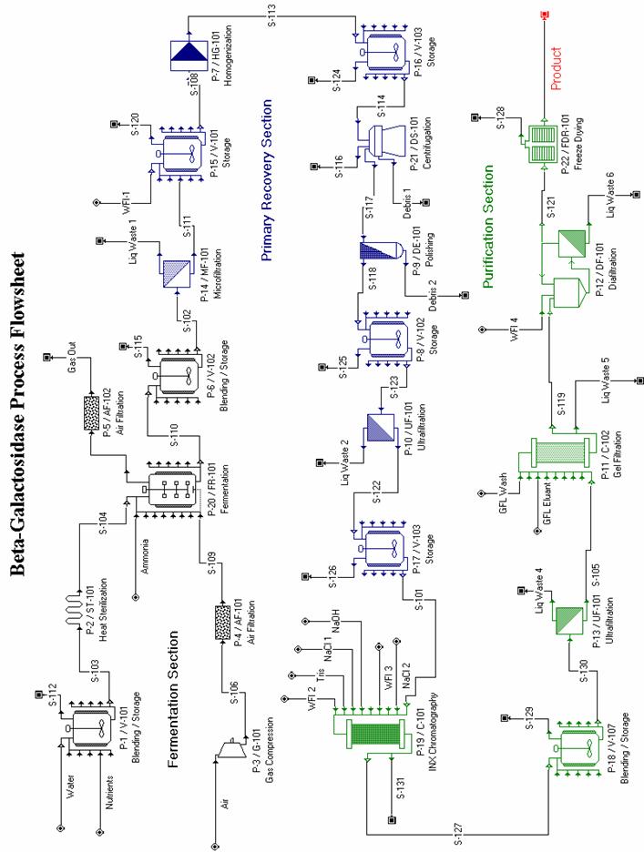
General note about Flowsheet Sections
The concept of flowsheet sections was introduced as part of release 3.0 to facilitate reporting of results for costing, economic evaluation, raw material requirements, and throughput analysis of integrated processes. A flowsheet section is a group of unit procedures that have something in common. For instance, the -galactosidase flowsheet has been divided into three sections: 1) Fermentation, 2) Primary Recovery, and 3) Purification. All the procedure icons of the Fermentation section are displayed in black, while the icons of the Primary Recovery and Purification sections are displayed in blue and green, respectively. If you wish to add unit procedures to a specific section, simply highlight the desired unit procedure icons on the flowsheet, and then click the Add to Section icon (the one with two blue triangles on it) on the left end of the Sections Toolbar. To specify the default color for icons in a specific section, click the Edit Section icon of the Sections Toolbar (this icon looks like a small pair of glasses and a piece of paper). This brings up a dialog box which allows you to specify a Starting Material and Active Product for the section. If you click on the Icon Color tab of this dialog, you can edit the sections default unit procedure icon color. These dialogs can also be reached by choosing Edit: Flowsheet Options: Section: Properties. For additional information on how to specify flowsheet sections and edit their properties, please consult the Help Facility (look up the keyword Sections in the Help index).
Fermentation Section
Fermentation media are prepared in a stainless steel tank (V-101) and sterilized in a continuous sterilizer (ST-101). A compressor (G-101) and an absolute air filter (AF-101) provide sterile air to the fermentor (FR-101). Gaseous ammonia is used as a nitrogen source.
Primary Recovery Section
The first step of the downstream section is cell harvesting to reduce the volume of the broth and remove extracellular impurities; it is carried out by a membrane microfilter (MF-101). Since ߖgalactosidase is an intracellular product, the next important step is cell disruption, performed in a high-pressure homogenizer (HG-101). Storage vessels (V-101, 102, 103, and 107) are used at various stages of the process to act as surge capacity for certain unit procedures with restricted throughputs. For instance, upstream of the P-7/HG-101 homogenizer is the P-15/V-101 storage vessel. This vessel is necessary because the time required for homogenization in HG-101 is greater than the time required for microfiltration in MF-101. Since these pieces of equipment do not have storage capacity within them, the difference in flow rates creates a necessity for intermediate storage equipment such as V-101. Notice that some of these vessels are used multiple times within the process (V-101, V-102, and V-103 are each used for two different steps.) After homogenization, a diskstack centrifuge (DS-101) is used to remove most of the cell debris particles. A dead-end polishing filter (DE-101) removes the remaining cell debris particles. The resulting protein solution is concentrated by an ultrafilter (UF-101), and stored in V-103.
Purification Section
Next the product stream is purified by an ion exchange chromatography column (C-101), further concentrated by a second ultrafiltration step (P-13/UF-101), and polished by a gel filtration column (C-102). Finally, a diafiltration unit (DF-101) exchanges the gel filtration buffer, and the protein solution is lyophilized in a freeze dryer (FDR-101).
In a batch plant, it is common to utilize the same piece of equipment to carry out multiple unit procedures. As stated above, vessels V-101, V-102, and V-103 are each used for multiple steps within this example process. Similarly, the ultrafilter, UF-101, is used twice. By default, whenever a unit procedure is introduced in the flowsheet, the system assumes that the procedure is carried out in its own piece of equipment. However, you also have the option of selecting one of the existing equipment items that are compatible with this unit procedure through the Equipment Data dialog (right-click on a unit procedure icon and choose the Equipment Data option).
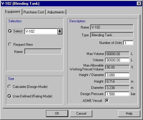
The figure above displays the equipment data dialog of procedure P-8. Instead of using a unique vessel for this procedure, vessel V-102 (which was first used for procedure P-6) was reused. Equipment sharing is possible in either Design or Rating mode. When multiple procedures share a piece of equipment that is in Design mode (unspecified size), each procedure recommends its own sizing and SuperPro selects the maximum. If the calculated equipment size exceeds the maximum possible value, then SuperPro assumes multiple (identical) equipment items with a total size equal to the calculated
total capacity requirement and an individual size that is smaller than or equal to the maximum. For example, if the maximum size of a vessel is 80,000 L, and your process requires 180,000 L of storage capacity, three 60,000 L vessels will be used by SuperPro. In Rating mode, the user specifies the equipment size as well as the number of equipment items employed by a unit procedure. In other words, in SuperPro a single unit procedure icon may correspond to multiple equipment items that operate in parallel, or multiple unit procedure icons may correspond to a single piece of equipment (if the flowsheet is in Batch mode and those procedures share equipment).
Equipment sharing reduces the number of equipment items required for a batch process and consequently saves money in terms of capital expenditures. However, it also introduces scheduling constraints that may reduce the number of batches that can be processed per year. Information on visualization of equipment sharing can be found later in this chapter. For detailed information on the impact of equipment sharing on plant throughput please search for Debottlenecking in the Help Facility.
In bioprocessing, we have formation of intracellular (remaining inside the cell) as well as extracellular (released into the solution) products. To capture this as well as the fact that biomass is usually reported on a dry-cell-mass basis, we use the concept of Extra-Cell % in streams and fermentation reactions. The Extra-Cell % of a component in an input stream (something fed into the system) or a product of a fermentation reaction (something generated in the system) can be specified only if the Primary Biomass Component is identified.
This is accomplished through the Pure Component Registration dialog (select Tasks: Register Components & Mixtures: Pure Components) shown in the figure below. The primary biomass component is selected among components whose Is Biomass? box has been checked (with an x) on the IDs tab of the Properties dialog. The Properties dialog is displayed by clicking on a components line number (# 3 for Biomass in the figure below) on the left-most column of the Registered Components table and then clicking on the Properties button.
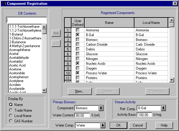
The Pure Component Registration dialog.
If the Primary Biomass Component is identified, its Water Content is specified (through the same dialog) and there is formation of Primary Biomass (as a fermentation product), the program will automatically associate intracellular water with biomass in order to satisfy its water content as specified during component registration. This is displayed using an Extra-Cell % value of less than 100 in the stream dialogs. This value has an impact on material balances in separation procedures (e.g., centrifugation, clarification, filtration, etc.). If a removal percentage is assigned to Primary Biomass, the program will use the same removal percentage for the intracellular portion of all components. This results in solids streams (e.g., retentate, centrate, etc.) with concentrations closer to reality.
Please note that a fermentation product can be identified as intracellular by specifying an Extra-Cell % value of less than 100 in the Stoichiometry tab of a fermentation operation dialog. That component can become extracellular (released into the solution) using a cell disruption procedure (e.g., high pressure homogenization or bead milling).
In bioprocessing, the concentration of a product or undesired impurity is often reported as activity measured using a certain assay. In SuperPro this is represented using the Stream Activity Reference Component and its Activity Basis, expressed in U/mg (see previous figure). The activity basis represents how many (arbitrary) units of activity (U) correspond to each mg of the reference component present in a stream. This information is used to calculate and report the activity of a stream in U/mL (see figure below). This concept is also applicable to other industries. For instance, in treatment of nuclear waste, the calculated stream activity may represent radioactivity.
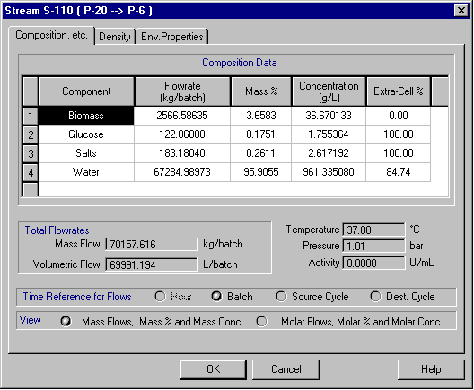
Dialog of stream S-110 (fermentation outlet).
Initializing Fermentation Operations
Correct modeling of fermentation operations is important in biotech processes. Pro-Designer is equipped with two different types of fermentation models: stoichiometric and kinetic. These operations can be utilized for batch as well as continuous fermentation reactions. The stoichiometric model is used if no kinetic data are available or if simplicity is desired, which is the case in this example. If kinetic data are available, the kinetic model can be used to calculate composition, temperature, and utility profiles as a function of time. Initialization of a stoichiometric fermentation is essentially identical to initialization of a stoichiometric chemical reaction, except that there is an option on the Fermentation Oper Conds tab for fermentor aeration. Please refer to Chapter4 for information on initialization of stoichiometric chemical reactions. Chapter 4 also provides information on initialization of kinetic reactions and generation of profiles as a function of time.
The calculated flowrates and compositions of intermediate and output streams can be viewed by revisiting the input/output dialog windows of each stream (double click on a stream line or click with the right mouse button and select Simulation Data). In addition, a report containing information on raw material requirements, stream compositions and flowrates, as well as an overall material balance, can be generated by selecting the Tasks: Generate Stream Report (SR) option from the main menu. The resulting report can be viewed by selecting the View: Stream Report option of the main menu. Tables 3a,b, and c display portions of the stream report. These tables were extracted from the spreadsheet version of the Stream Report, which was generated by selecting File : Export Reports to Excel. They were then edited in Excel and pasted into SuperPro as a MS Excel worksheet.
Table 3a: Overall Process Data

MP = Main Product
Table 3b: Starting Material Requirements

Table 3c: Raw Material Requirements Entire Flowsheet

SuperPro generates Operations and Equipment Gantt charts for single and multiple batches. The figure below displays a portion of the operations Gantt chart for a single batch of this example process.
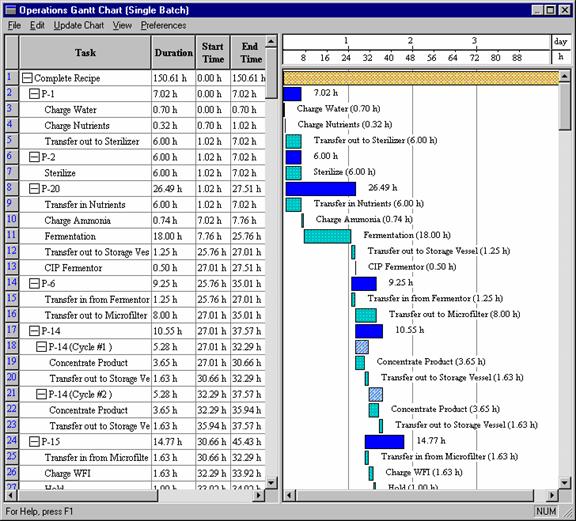
The Operations Gantt Chart for a Single Batch.
The left view (spreadsheet view) displays the name, duration, start time, and end time for each activity (e.g. each operation, unit procedure, cycle, batch, etc). You can use the left view to expand or collapse the activity summaries by clicking on the + or signs in the boxes to the left of the activity names.
The right view (chart view) displays a bar for each activity in the overall process recipe. To edit the scheduling data (or any other data affecting an activity), simply right-click on a bar and a relevant command menu will appear. Selecting the uppermost entry on this menu will bring up a dialog that will allow you to edit the information associated with that particular activity bar. In fact, anything you can accomplish with the other scheduling interfaces, you can also accomplish from the Gantt chart interface. Furthermore, you can redo the M&E balances and have the Gantt Chart updated to reflect the new (calculated) scheduling settings for the recipe by clicking on the Update Chart entry in the main menu of the interface.
Another way of visualizing the execution of a batch process as a function of time is through the Equipment Utilization chart (select View : Equipment Utilization Chart). The figure below displays the equipment utilization chart for two consecutive batches of this example process. Multiple bars on the same line (e.g., for V-101, V-102, V-103, and UF-101) represent reuse (sharing) of equipment by multiple procedures. White space represents idle time. The equipment with the least idle time between consecutive batches is the time (or scheduling) bottleneck (C-101 in this case) that determines the maximum number of batches per year. Its occupancy time (approximately 56 hours) is the minimum possible time between consecutive batches (also known as Min. Effective Plant Batch Time). The actual time between consecutive batches (also known as Effective Plant Batch Time) is approximately 58.2 hours. The plant batch time (the time required to complete a single batch) is roughly 150 hours.
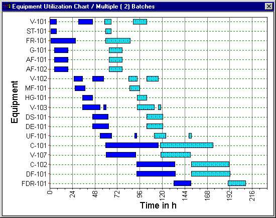
The Equipment Utilization Chart (two consecutive batches).
SuperPro also generates utilization charts for auxiliary equipment, such as clean-in-place (CIP) and steam-in-place (SIP) skids.
In addition to creating Gantt charts for equipment utilization and operations, SuperPro Designer automatically generates graphs of resource demand as a function of time for such things as heating and cooling utilities, power, labor, and raw materials. To view these graphs, select View: Resource Chart, and then choose the desired resource from the drop-down menu. The figure below displays the water for injection (WFI) demand graph for four consecutive batches. Demand for WFI and clean steam are common bottlenecks in biomanufacturing facilities.
SuperPro is equipped with powerful throughput analysis and debottlenecking capabilities. The objective of these features is to allow the user to quickly and easily analyze the capacity and time utilization of each piece of equipment, and to identify opportunities for increasing throughput with the minimum possible capital investment. For a detailed throughput analysis example, please see Chapter 6 or search for Debottlenecking in the Help Facility.
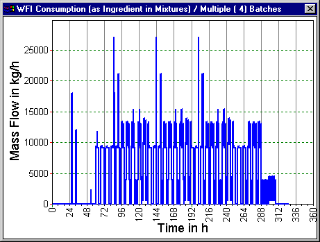
WFI Demand Chart (four consecutive batches).
Several different economic reports can be generated from SuperPro Designer. To view the essential economic evaluation results for the whole process, please select View: Executive Summary. You will need to generate the Economic Evaluation Report (EER) and the Itemized Cost Report (ICR) if you wish to view the detailed results. Portions of the EER and ICR appear on the following pages.
The Economic Evaluation Report (EER)
This report provides information on the capital investment and operating costs for the entire flowsheet. It also includes profitability and cash-flow analysis tables. Additional cost data, broken down per section, is available in the Itemized Cost Report (which follows the EER tables).
To generate the EER, select Tasks: Generate Economic Evaluation Report. To view it, select View: Economic Evaluation Report. Like the stream report, the economic evaluation report is a text file which may be read by a variety of text editors and word processors. The same report (like any other report) can also be generated in spreadsheet format by selecting File: Export Reports to Excel. The EER for the b-Galactosidase design case begins on the next page.
Economic Evaluation Report (EER) for the BGal4_0b Design File
The EER provides summaries and detailed breakdowns of various factors which affect the overall capital investment and the operating cost. Additional cost data, broken down per section, are available in the Itemized Cost Report (which follows the EER tables).

EXECUTIVE SUMMARY (1999 prices)
TOTAL CAPITAL INVESTMENT 63386000 $
CAPITAL INV. CHARGED TO THIS PROJECT 63386000 $
OPERATING COST 34922000 $/year
PRODUCTION RATE 11538 kg/year of B-Gal (in Product)
UNIT PRODUCTION COST 3027 $/kg of B-Gal (in Product)
TOTAL REVENUES 63462000 $/year
GROSS MARGIN 44.97 %
RETURN ON INVESTMENT 35.84 %
PAYBACK TIME 2.79 years
IRR AFTER TAXES 24.14 %
NPV (at 7.0 % interest) 79127000 $

MAJOR EQUIPMENT SPECIFICATION AND FOB COST (1999 prices)
Quantity/ Description Unit Cost Cost
Stand-by ( $ ) ( $ )
1/0 ST-101 Heat Sterilizer 361000 361000
Diameter = 7.50 m
Length = 5.55 m
1/0 V-101 Blending Tank 287000 287000
Volume = 80000.00 L
Diameter = 3.24 m
1/0 G-101 CF Compressor 188000 188000
Power = 235.52 kW
1/0 AF-101 Air Filter 4000 4000
Rated Throughput = 0.13 m^3/s
To keep this manual concise, most of the equipment listed in the EER was deleted from this table. If you wish to see the entire table, please open the BGal4_0b.spf example and generate the EER. ****
2/0 FDR-101 Freeze Dryer 1491000 2982000
Tray Area = 6.01 m2
Capacity = 453.08 kg H2O/cycle
Cost of Unlisted Equipment 1989000
TOTAL EQUIPMENT PURCHASE COST 9946000
Economic Evaluation Report (continued)

FIXED CAPITAL ESTIMATE SUMMARY (1999 prices)
A. TOTAL PLANT DIRECT COST (TPDC) (physical cost)
1. Equipment Purchase Cost $ 9946000
2. Installation 3347000
3. Process Piping 3481000
4. Instrumentation 3978000
5. Insulation 298000
6. Electricals 995000
7. Buildings 4476000
8. Yard Improvement 1492000
9. Auxiliary Facilities 3978000
----- ----- --------------
TPDC = 31992000
B. TOTAL PLANT INDIRECT COST (TPIC)
10. Engineering 7998000
11. Construction 11197000
----- ----- --------------
TPIC = 19195000
C. TOTAL PLANT COST (TPDC+TPIC) TPC = 51186000
12. Contractor's fee 2559000
13. Contingency 5119000
----- ----- --------------
(12+13) = 7678000
D. DIRECT FIXED CAPITAL (DFC) TPC+12+13 = 58864000

LABOR REQUIREMENT AND COST SUMMARY
Section Labor Hours Labor Cost
Name Per Year $/year %
Fermentation Secti 12689 759000 18.86
Primary Recovery S 24521 1466000 36.44
Purification Secti 30085 1799000 44.71
TOTAL 67295 4024000 100.00
Economic Evaluation Report (continued)

RAW MATERIALS COST SUMMARY
Raw Unit Cost Annual Amount Cost
Material ( $/kg ) ( kg ) ( $/yr ) %
Process Water 0.010 8576000.00 85760 0.67
Glucose 1.000 823162.00 823162 6.48
Salts 1.600 137484.00 219974 1.73
Ammonia 0.500 52930.00 26465 0.21
WFI 0.100 31972978.25 3197298 25.16
Tris Buffer 0.150 25258404.94 3788761 29.82
NaCl (0.1 M) 0.130 20692755.04 2690058 21.17
NaOH (0.5 M) 0.120 12761902.29 1531428 12.05
NaCI (0.5 M) 0.190 1806726.64 343278 2.70
TOTAL 102082343.16 12706000 100.00

VARIOUS CONSUMABLES (1999 prices)
MEMBRANE or FILTER CLOTH
Procedure Equipment Unit Cost Annual Amount Cost
Name Name ( $/m^2 ) ( m^2 ) ( $/yr )
P-9 DE-101 12.00 26800.00 322000
P-10 UF-101 200.00 133.64 27000
P-12 DF-101 250.00 41.51 10000
P-13 UF-101 200.00 26.37 5000
P-14 MF-101 200.00 169.68 34000
SUBTOTAL 398000
CHROMATOGRAPHY RESINS
Procedure Equipment Unit Cost Annual Amount Cost
Name Name ( $/L ) ( L ) ( $/yr )
P-11 C-102 200.00 17540.56 3508000
P-19 C-101 200.00 8419.47 1684000
SUBTOTAL 5192000
TOTAL 5590000
Economic Evaluation Report (continued)

WASTE TREATMENT / DISPOSAL (1999 prices)
a. SOLID WASTE
Stream Unit Cost Annual Amount Cost
Name ( $/kg ) ( kg ) ( $/yr )
a. Subtotal (Solid Waste) 0
b. LIQUID WASTE
Stream Unit Cost Annual Amount Cost
Name ( $/kg ) ( kg ) ( $/yr )
Debris 2 1.000e-002 202075.82 2000
Liq Waste 2 1.000e-002 3392864.25 34000
Liq Waste 6 1.000e-002 1337718.30 13000
Liq Waste 5 1.000e-002 20538100.51 205000
Liq Waste 1 1.000e-002 4692478.85 47000
Debris 1 1.000e-002 68857.43 1000
Liq Waste 4 1.000e-002 519741.94 5000
b. Subtotal (Liquid Waste) 307000
c. EMISSIONS
Stream Unit Cost Annual Amount Cost
Name ( $/kg ) ( kg ) ( $/yr )
c. Subtotal (Emissions) 0
WASTE TREATMENT/DISPOSAL TOTAL COST (a+b+c) 308000
Economic Evaluation Report (continued)

UTILITY REQUIREMENTS (1999 prices)
ELECTRICITY
Procedure Equipment Annual Amount Cost
Name Name ( kWh ) ( $/yr )
P-3 G-101 441838 44184
P-7 HG-101 313002 31300
P-10 UF-101 33905 3391
P-12 DF-101 23370 2337
P-13 UF-101 10338 1034
P-14 MF-101 46894 4689
P-20 FR-101 498986 49899
P-21 DS-101 40512 4051
P-22 FDR-101 25750 2575
Unlisted Equipment 89662 8966
General Load 268987 26899
SUBTOTAL 179324
HEAT TRANSFER AGENT : Steam (0.2800 $/1000 kg)
Procedure Equipment Annual Amount Cost
Name Name ( kg ) ( $/yr )
P-22 FDR-101 259044 73
SUBTOTAL 282
HEAT TRANSFER AGENT : Cooling Water (0.0250 $/1000 kg)
Procedure Equipment Annual Amount Cost
Name Name ( kg ) ( $/yr )
SUBTOTAL 1324
HEAT TRANSFER AGENT : Chilled Water (0.1750 $/1000 kg)
Procedure Equipment Annual Amount Cost
Name Name ( kg ) ( $/yr )
P-3 G-101 38722304 6776
P-7 HG-101 67628398 11835
P-10 UF-101 621337 109
P-12 DF-101 377116 66
P-13 UF-101 1681399 294
P-14 MF-101 23112113 4045
P-20 FR-101 394140398 68975
P-21 DS-101 6973328 1220
SUBTOTAL 93320
TOTAL 272644
Economic Evaluation Report (continued)

ANNUAL OPERATING COST - SUMMARY (1999 prices)
Cost Item $/Year %
Raw Materials 12706000 36.38
Labor-Dependent 4024000 11.52
Equipment-Dependent 11097000 31.78
Laboratory/QC/QA 925000 2.65
Consumables 5590000 16.01
Waste Treatment/Disposal 308000 0.88
Utilities 273000 0.78
Transportation 0 0.00
Miscellaneous 0 0.00
Advertising and Selling 0 0.00
Running Royalties 0 0.00
Failed Product Disposal 0 0.00
TOTAL 34922000 100.00

PROFITABILITY ANALYSIS (1999 prices)
A. DIRECT FIXED CAPITAL $ 58864000
B. WORKING CAPITAL 1578000
C. STARTUP COST 2943000
D. UP-FRONT R&D 0
E. UP-FRONT ROYALTIES 0
F. TOTAL INVESTMENT (A+B+C+D+E) 63386000
G. INVESTMENT CHARGED TO THIS PROJECT 63386000
H. REVENUE STREAM FLOWRATES
kg/year of B-Gal (in Product) 11538
I. PRODUCTION (UNIT) COST
$/kg of B-Gal (in Product) 3026.576
J. SELLING/PROCESSING PRICE
$/kg of B-Gal (in Product) 5555.556
K. REVENUES ($/year)
Product 63462000
L. ANNUAL OPERATING COST 34922000
M. GROSS PROFIT (K-L) 28540000
N. TAXES (40 %) 11416000
O. NET PROFIT (M-N + Depreciation ) 22716000
GROSS MARGIN 44.97 %
RETURN ON INVESTMENT 35.84 %
PAYBACK TIME (years) 2.79
Economic Evaluation Report for the Design File BGal4_0b (cont.)
|
CASH
FLOW ANALYSIS (thousand | |||||||||||
|
YR |
CAPITAL |
DEBT |
SALES |
OPERAT. |
GROSS |
LOAN |
DEPREC |
TAXABLE |
TAXES |
NET |
NET |
|
INVESTM |
FINANCE |
COST |
PROFIT |
PAYMENT |
INCOME |
PROFIT |
CASH FLOW |
||||
|
| |||||||||||
|
IRR BEFORE TAXES |
% |
INTEREST | |||||||||
|
IRR AFTER TAXES |
% |
NPV | |||||||||
|
Depreciation Method: |
Straight-Line | ||||||||||
|
DFC Salvage Factor | |||||||||||
Itemized Cost Report (ICR) for the BGal4_0b Design File
The Itemized Cost Report (ICR) provides detailed operating cost data, broken down per flowsheet section and cost item. It enables the user to readily identify the cost sensitive sections of a process the economic hot-spots. For instance, a quick look at the following tables reveals that the Purification section is the most expensive part of this process. In particular, raw materials and equipment contribute large amounts to the overall expense of the project. Thus it would be wise to allocate resources to optimize this section, as opposed to using those same resources elsewhere where optimization would have little effect on the overall project cost. A look back at the Economic Evaluation Report reveals the cost of each individual piece of equipment, as well as the costs for installation, piping, instrumentation, etc. The user should look at each of these expenses to ensure they are accurate for their particular application. For instance, if no auxiliary facilities need to be constructed, or if the required freeze dryers can be shared with another process, the overall cost will be significantly reduced. Another potential economic hotspot is the high cost of raw materials, notably the WFI and buffer solutions. Perhaps the quantities of these materials could be reduced.
The above analysis shows how the economic reports can be used not only for estimation of the total cost of a process, but also as a tool to optimize the process through what-if scenarios. Would it make economic sense to use a less expensive chromatography resin if it required more cycles to be run and more buffer solution to be used? It depends on how many more cycles are needed, and how much cheaper the new resin is. Would a radically modified purification scheme be better than the current scheme? It depends on what equipment, reagents, etc. would be required for the modified purification, and what the overall yield of the product would be. This type of what-if analysis is quick and easy to perform using SuperPro Designer.
To generate the Itemized Cost Report, select Tasks: Generate Itemized Cost Report. To view the report, select View: Itemized Cost Report. A portion of the Itemized Cost Report for the b-galactosidase case follows.
Itemized Cost Report (continued)

FLOWSHEET PARAMETERS
Operating Time = 7897 (h/yr)
Main Product Rate = 11538 (kg/yr)
Plant Batch Time = 151 (h)
Effective Plant Batch Time = 58 (h)
Number of Batches Per Year = 134

COST PER FLOWSHEET SECTION (1999 prices)
SECTIONS IN: Main Branch
Fermentation Section Sin = Glucose Aout = Biomass
Cost Item $/kg MP $/Batch $/Year %
Raw Materials 100.131 8622 1155361 26.78
Equipment 170.935 14719 1972330 45.72
Labor 65.761 5663 758781 17.59
Consumables 0.000 0 0 0.00
Lab/QC/QA 20.323 1750 234500 5.44
Waste Trtm/Disp 0.000 0 0 0.00
Utilities 16.757 1443 193354 4.48
Transportation 0.000 0 0 0.00
Miscellaneous 0.000 0 0 0.00
Section Total 373.908 32196 4314326 100.00
Primary Recovery Section Sin = Biomass Aout = B-Gal
Cost Item $/kg MP $/Batch $/Year %
Raw Materials 20.394 1756 235313 4.85
Equipment 198.141 17062 2286242 47.17
Labor 127.086 10943 1466384 30.25
Consumables 33.130 2853 382265 7.89
Lab/QC/QA 27.872 2400 321600 6.64
Waste Trtm/Disp 7.242 624 83563 1.72
Utilities 6.196 534 71498 1.48
Transportation 0.000 0 0 0.00
Miscellaneous 0.000 0 0 0.00
Section Total 420.061 36171 4846864 100.00
Purification Section Sin = B-Gal Aout = B-Gal
Cost Item $/kg MP $/Batch $/Year %
Raw Materials 980.676 84444 11315510 43.93
Equipment 592.659 51033 6838385 26.55
Labor 155.921 13426 1799086 6.98
Consumables 451.330 38863 5207657 20.22
Lab/QC/QA 31.937 2750 368500 1.43
Waste Trtm/Disp 19.409 1671 223956 0.87
Utilities 0.675 58 7793 0.03
Transportation 0.000 0 0 0.00
Miscellaneous 0.000 0 0 0.00
Section Total 2232.607 192245 25760886 100.00
Itemized Cost Report (continued)

SUMMARY (Entire Flowsheet)
Cost Item $/kg MP $/Batch $/Year %
Raw Materials 1101.201 94822 12706184 36.38
Equipment 961.735 82813 11096956 31.78
Labor 348.768 30032 4024251 11.52
Consumables 484.459 41716 5589922 16.01
Lab/QC/QA 80.132 6900 924600 2.65
Waste Trtm/Disp 26.652 2295 307518 0.88
Utilities 23.629 2035 272644 0.78
Transportation 0.000 0 0 0.00
Miscellaneous 0.000 0 0 0.00
Flowsheet Total 3026.576 260613 34922076 100.00
Sin = Section Starting Material
Aout = Section Active Product
MP = Main Product (of the entire flowsheet)

BREAKDOWN PER COST ITEM AND SECTION
Cost Item Fermentatio Primary Rec Purificatio Subtotal %
$/year $/year $/year $/year
Raw Materials 1155361 235313 11315510 12706184 36.38
Equipment 1972330 2286242 6838385 11096956 31.78
Labor 758781 1466384 1799086 4024251 11.52
Consumables 0 382265 5207657 5589922 16.01
Lab/QC/QA 234500 321600 368500 924600 2.65
Waste Trt/Dsp 0 83563 223956 307518 0.88
Utilities 193354 71498 7793 272644 0.78
Transportation 0 0 0 0 0.00
Miscellaneous 0 0 0 0 0.00
Subtotal 4314326 4846864 25760886 34922076 100.00
Contribution (%) 12.35 13.88 73.77 100.00

RAW MATERIALS COST BREAKDOWN (Values in $/year)
Raw Material Fermentation Primary Recov Purification Subtotal %
Process Water 85760 0 0 85760 0.67
Glucose 823162 0 0 823162 6.48
Salts 219974 0 0 219974 1.73
Ammonia 26465 0 0 26465 0.21
WFI 0 235313 2961984 3197298 25.16
Tris Buffer 0 0 3788761 3788761 29.82
NaCl (0.1 M) 0 0 2690058 2690058 21.17
NaOH (0.5 M) 0 0 1531428 1531428 12.05
NaCI (0.5 M) 0 0 343278 343278 2.70
TOTAL 1155361 235313 11315510 12706184 100.00
Contribution (%) 9.09 1.85 89.06 100.00
The Environmental Impact Report provides information on the amount and type of waste generated by a manufacturing or waste treatment facility. It also provides information on the fate of a compound that enters an integrated manufacturing or waste treatment facility. To create the environmental impact report select Tasks: Generate Environmental Impact Report (EIR). To view this report, select View: Environmental Impact Report.
SuperPro Designer contains a variety of formulation, packaging, and transportation unit procedures in order to capture the cost associated with such processes.
Product formulation and packaging processes often involve formation and use of discrete entities, such as tablets, bottles, boxes, etc. The flow of such entities is represented by discrete streams, which by default are displayed in blue. For more information on discrete streams and entities, please consult the Help Facility.
To familiarize yourself with the formulation and packaging models and the concepts of discrete streams and entities, please open the BGal4_0c.spf design case in the EXAMPLESBGAL folder and visit the simulation data dialog windows of those operations. As usual, you can open these dialogs by right-clicking on the various packaging unit procedure icons and their corresponding streams. Notice the different interface of discrete streams, which display the flow of discrete entities as well as the equivalent bulk flow (based on the bulk ingredients that compose the discrete entities).
This chapter briefly describes how to use the demonstration program to develop and analyze a flowsheet for the production of a synthetic pharmaceutical intermediate. This example is recommended for users in the pharmaceutical, agrochemical, and specialty chemical industries. A more detailed description can be found in EXAMPLESSYNPHARMSYNPHARM.DOC.
Several reaction and separation steps are required to synthesize and purify the pharmaceutical intermediate product. The generation of the flowsheet was based on information available in the patent and technical literature. The seven Pro-Designer files that are included in this example can be found in the Examples Synpharm subdirectory:
File SPhr4_0L: This process is based on lab-scale data which has been scaled up to pilot plant production volumes. At this point all equipment is in Design Mode. In other words, the equipment capacities have not yet been fixed.
File SPhr4_0a: This process was designed based on pilot plant volumes of reagents in manufacturing scale equipment. It is the same as SPhr4_0L except that the calculation mode for all process steps has been switched to Rating Mode. In addition, the reactors and filter are used for multiple unit procedures. Two 1000 gal reactors, one 4 m2 filter and one 10 m2 tray dryer are utilized.
File SPhr4_0b: This process is the same as SPhr4_0a, but the throughput has been scaled to 100% capacity utilization of the limiting-size reactor (R-102).
File SPhr4_0c: This process is the same as SPhr4_0b, except that THREE reactors are used in order to decrease the plants effective batch time (so that more cycles can be run per year).
File SPhr4_0d: This process is the same as SPhr4_0c except that a second filter (NFD-102) has been added.
File SPhr4_0e: This is the same as SPhr4_0d except that procedure P-11 in R-103 (and subsequent procedures) have been split into two cycles, and the batch throughput has been increased to 100% in the new capacity-limiting piece of equipment (R-102).
File SPhr4_0f: This is the same as SPhr4_0e except that the utilization of several reactors has been rearranged. Specifically, the reactors for procedures P-5 and P-7 have been switched. This allows more cycles to be run per year because the batch cycle time of reactor R-103 is decreased. The SPhr4_f file is described in more detail below.
The description that follows corresponds to SPhr4_0f (see figure on next page). Please open this file now. The objective is to produce at least 33,000 kg of this intermediate per year in a plant that has the following equipment items:
1) three stirred-tank reactors each having a total volume of 1000 gallons,
2) two nutsche filters each with an area of 4 m2, and
3) a tray dryer with a total tray area of 10 m2.
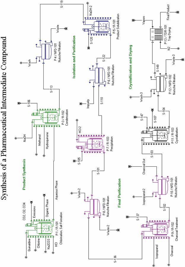
Chlorination Reaction and Salt Formation Steps (P-1/R-101)
The first reaction step involves the chlorination of quinaldine. Quinaldine is dissolved in carbon tetrachloride (CCl4) and reacts with gaseous Cl2. The yield of the reaction is around 98%. The generated HCl is neutralized using Na2CO3. The stoichiometry and yield of the three reactions follows:
Quinaldine + Cl ===> Chloroquinaldine + HCl Yield = 98 %
Na CO + HCl ===> NaHCO + NaCl Yield = 100 %
NaHCO + HCl ===> NaCl + H O + CO Yield = 100 %
Small amounts of unreacted Cl2, generated CO2, and volatilized CCl4 are vented. The above three reactions occur sequentially in the first reactor vessel (R-101).
The second reaction step involves the formation of Chloroquinaldine.HCl. The added HCl first neutralizes the remaining NaHCO3 and then reacts with chloroquinaldine to form its salt. The stoichiometry and yield of the two reactions follows:
NaHCO + HCl ===> NaCl + H O + CO Yield = 100 %
Chloroquinaldine + HCl ===> Chloroquinaldine.HCl Yield = 100 %
Small amounts of generated CO2 and volatilized CCl4 are vented. The presence of water (added with HCl as hydrochloric acid solution) and CCl4 leads to the formation of two liquid phases. The small amounts of unreacted quinaldine and chloroquinaldine remain in the organic phase while the salts Chloroquinaldine.HCl and NaCl move to the aqueous phase. After the reactor contents have been allowed to settle, the aqueous phase is transferred to R-102 for further processing. The organic phase is then discharged as waste. Approximately 15.8 hours are required for the chlorination and salt formation reactions above, along with all associated charges and transfers. (Note the times given for other procedures below also include associated material transfers, etc.)
Condensation Reaction Step (P-3/R-102)
The third reaction step involves the condensation of chloroquinaldine and hydroquinone. First, the salt chloroquinaldine.HCl is converted back to chloroquinaldine using NaOH. Then, hydroquinone reacts with NaOH and yields hydroquinone.Na. Finally, chloroquinaldine and hydroquinone.Na react and yield the desired intermediate product. Along with product formation, a small amount of chloroquinaldine dimerizes and forms an undesirable by-product (Impurity) that needs to be removed from the product. The stoichiometry and yield of the four reactions follows:
Chloroquinaldine.HCl + NaOH ===> NaCl + H O + Chloroquinaldine Yield = 100 %
2Chloroquinaldine + 2NaOH ===> 2H O + 2NaCl + Impurity Yield = 2 %
Hydroquinone + NaOH ===> H O + Hydroquinone .Na Yield = 100 %
Chloroquinaldine + Hydroquinone.Na ===> Product + NaCl Yield = 100 %
This step takes a total of 16.3 hours to complete.
Filtration Step #1 (P-4/NFD-101)
Both the product and impurity molecules formed during the condensation reaction precipitate out of solution and are recovered using a nutsche filter. The product recovery yield is 90%. The total filtration and cake discharge time is 5.4 hours assuming an average filtrate flux of 200 L/m2-h.
Solubilization Reaction Step (P-5/R-101)
The Product/Impurity cake recovered by filtration is added into a NaOH solution. The Product molecules react with NaOH forming Product.Na which is soluble in water. The Impurity molecules remain in solid phase. The stoichiometry and yield of the solubilization reaction follows:
Product + NaOH ===> H O + Product.Na Yield = 100 %
This step takes a total of 10.9 hours.
Filtration Step #2 (P-6/NFD-101)
Next the Impurity is removed using another filtration step (NFD-101). The total filtration and cake discharge time is 3.5 hours assuming an average filtrate flux of 200 L/m2-h.
Precipitation Reaction Step (P-7/R-103)
The excess NaOH is neutralized using HCl and then Product.Na is converted back to Product. The stoichiometry and yield of the two reactions follows:
HCl + NaOH ===> H O + NaCl Yield = 100 %
HCl + Product .Na ===> NaCl + Product Yield = 100 %
The Product, which is insoluble in water, precipitates out of solution. This step takes around 8.1 hours.
Filtration Step #3 (P-8/NFD-101)
Next the Product is recovered using another filtration step. The Product cake is washed with water to remove impurities. The product recovery yield is 90%. The filtration and cake discharge time is 4.8 hours assuming an average filtrate flux of 200 L/m2-h.
Charcoal Treatment (P-9/R-102)
The recovered Product cake is solubilized in isopropanol and treated with charcoal for discoloration. This step takes a total of 17.6 hours.
Filtration Step #4 (P-10/NFD-101)
After charcoal treatment, the solid carbon particles are removed using another filtration step. The filtration and cake discharge time is around 14.8 hours assuming an average filtrate flux of 200 L/m2-h, and a hold time of 10.4 hours (to account for the extra time spent waiting for the second filtration cycle to get underway).
Crystallization Step (P-11/R-103)
In this step, the product solution is distilled to one third of its initial volume. Then it is crystallized with a yield of 97%. Crystallization is represented by the following reaction:
Product ===> Product-Cryst Yield = 97 %
In other words, a new component (Product-Cryst) is used to represent the crystalline form of product. This step is performed in two 12.1 hour cycles.
Filtration Step #5 (P-12/NFD-102)
The crystalline product is recovered using another filtration step with a yield of 90%. The filtration and cake discharge takes place in two 12.1 hour cycles, assuming an average filtrate flux of 50 L/m2-h, and an 8.5 hour hold time (the hold time is necessary to synchronize these cycles with the P-11 crystallization step cycles).
Drying Step (P-13/TDR-101)
The recovered product crystals are dried in a tray dryer. The drying is done in two 12.1 hour cycles, which includes a 3.02 hour hold time (to synchronize these cycles with P-11 and P-12). Approximately 246 kg of dried product is produced per batch.
In a batch plant, it is common to utilize the same piece of equipment for carrying out multiple unit procedures. For instance, in this example process, vessel R-101 handles procedures P-1 and P-5. By default, whenever a unit procedure is introduced in the flowsheet, the system assumes that the procedure is carried out in its own piece of equipment. However, you also have the option of selecting one of the existing equipment items that are compatible with this procedure through the Equipment Data dialog (right-click on a unit procedure icon and choose the Equipment Data option).
The figure below displays the equipment data dialog of procedure P-5. Instead of using a unique vessel for this procedure, the user decided to reuse R-101, which also handles procedure P-1. Starting with version 4.0, equipment sharing is available in Design as well as in Rating mode.
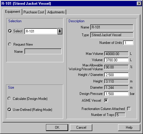
When multiple procedures share a piece of equipment that is in Design mode (unspecified size), each procedure recommends its own sizing and SuperPro selects the maximum. If the calculated equipment size exceeds the maximum possible value, then SuperPro assumes multiple (identical) equipment items with a total size equal to the calculated total capacity requirement and an individual size that is smaller than or equal to the maximum. For example, if the maximum size of an individual filter in Design mode is 5 m2, and your process requires 12 m2 of filter area to achieve the necessary throughput, three 4 m2 filters will be used by SuperPro. In Rating mode, the user specifies the equipment size as well as the number of equipment items employed by a unit procedure. In other words, in SuperPro a single unit procedure icon may correspond to multiple equipment items that operate in parallel, or multiple unit procedure icons may correspond to a single piece of equipment (if the flowsheet is in Batch mode and those procedures share equipment).
Equipment sharing reduces the number of equipment items required for a batch process and consequently saves money in terms of capital expenditures. However, it also introduces scheduling constraints that may reduce the number of batches that can be processed per year. Information on visualization of equipment sharing can be found in section 4.5. For detailed information on the impact of equipment sharing on plant throughput please see Chapter 6 or search for Debottlenecking in the Help Facility.
A flowsheet section is a group of process steps that have something in common. The flowsheet of this example was divided into four sections: 1) Product Synthesis, 2) Isolation and Purification, 3) Final Purification, and 4) Crystallization and Drying. All the process step icons of the Product Synthesis section are displayed in green. The icons in the Isolation and Purification, Final Purification, and Crystallization and Drying sections are displayed in blue, purple, and black, respectively. The molar yields of the Product Synthesis, Isolation and Purification, Final Purification, and Crystallization and Drying sections are 93.9%, 89.9%, 90.0%, and 87.3%, respectively. To view these yields, select the appropriate section through the drop-down menu of the section toolbar and then click on the 'Edit Section' button (the button with the pair of glasses). For more information on how to specify flowsheet sections and edit their properties, please consult the Help Facility.
Batch reactions constitute the most common operation in synthetic pharmaceutical processes. Pro-Designer is equipped with three different batch reaction operation models: stoichiometric, kinetic, and equilibrium. The stoichiometric is used if no kinetic and equilibrium data are available. If kinetic data are available, the kinetic model can be used to calculate composition, temperature, and utility profiles as a function of time. All reaction operations share the same Oper.Conds tab (see figure below) through which the user can specify the duration of the operation, the thermal mode, the power consumption, etc.
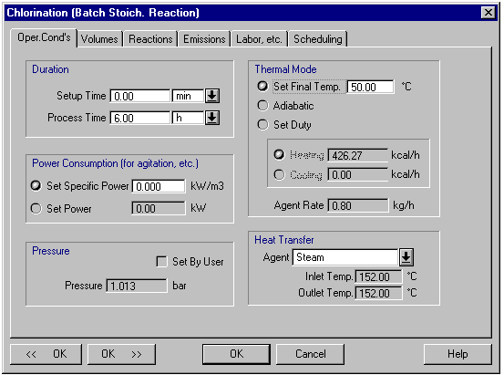
The Oper. Conds tab of a reaction operation.
Similarly, all reaction operations share the same Volumes tab (see figure below). In Design Mode (equipment size unspecified), the Maximum Allowable Working / Vessel Volume (%) value is used for sizing the vessel. If multiple operations in the same unit procedure require different capacity values, the maximum capacity requirement of these operations is selected as the equipment size. In Rating mode (equipment size specified), the Maximum Allowable (%) acts as a constraint that generates a warning when it is violated. The Minimum Allowable (%) value also acts as a constraint. The same logic applies to other vessel operations.
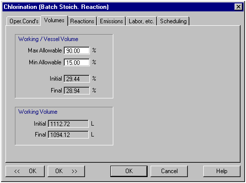
The Volumes tab of a reaction operation.
The figure below displays the Reactions tab of a stoichiometric reaction operation. Through this tab the user specifies the stoichiometry and other data associated with the various reactions in this operation. Please note that a reaction operation can handle any number of reactions.
The Extent of a stoichiometric reaction represents the fractional conversion of its limiting component. By default, the limiting component is identified by the model based on the stoichiometric coefficients and the feed composition. The user has the option to identify a reference component for the extent of reaction. In that case, if the specified value of the extent of reaction is not feasible, the model adjusts its value to the maximum possible. The user also has the option to specify the desired final concentration of a reactant or product and have the model estimate the extent of reaction. Again, in this case if the specified concentration is not feasible, the model adjusts its value to the maximum (or minimum) possible.
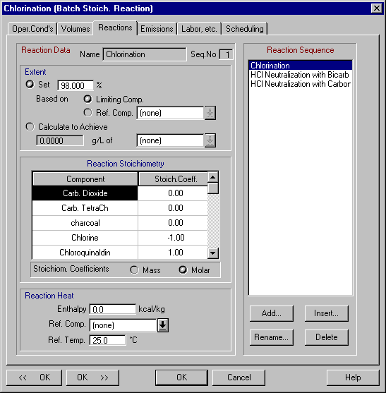
The Reactions tab of a stoichiometric reaction operation.
The Reactions tab of kinetic and equilibrium batch reactions is quite similar to that of the figure below. The main difference is that instead of the extent of reaction variables, it has a button through which the user can bring up the kinetic data dialog of a reaction (see next figure). Through this dialog the user specifies the kinetics of a reaction. Furthermore, clicking on the Start/End Criteria buttons brings up other dialogs through which the user can specify when or under what conditions a reaction is initiated or terminated.
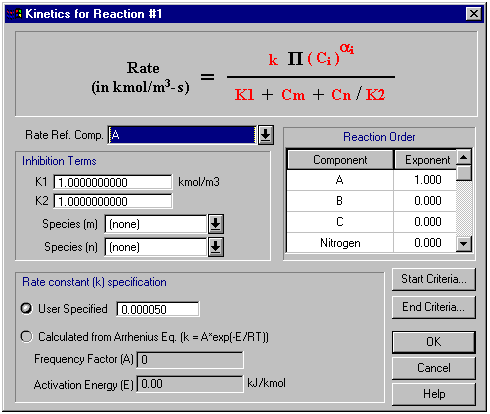
The Kinetics dialog of a kinetic reaction operation.
 Important
Note about Stoichiometric Reactions
Important
Note about Stoichiometric Reactions
Several different methods can be used to specify multiple reactions within a single Reaction Operation. For instance, each reaction could be written individually (as was done for the Chlorination and HCL Neutralizations listed in the Reaction Sequence box of the Chlorination operation Reactions tab shown previously.) In this case, mass balances for each reaction are performed sequentially. In other words, first the Chlorination Reaction proceeds to its specified Extent of Reaction. Then the first Neutralization proceeds to its specified Extent of Reaction. Finally, the second Neutralization occurs. In other situations, you may wish to specify reactions that occur simultaneously. This can be done several ways. In the first method, you can specify all stoichiometric coefficients in one reaction. Consider the following example: 90% of your Starting Material reacts with your Reagent to produce the Desired Product, while the other 10% self-couples to form a Byproduct (made of two reagent molecules):
Starting Material + Reagent à Desired Product (90% yield)
Starting Material + Starting Material à Byproduct
These two scenarios would happen simultaneously, and the extent of reaction for this system would be 100% (100% of the Starting Material would react). In this situation, the relative stoichiometric coefficients (on a molar basis) of Starting Material, Reagent, Desired Product, and Byproduct would be: -1, -0.9, 0.9, and 0.05, respectively. In other words, for every 1 mole of Starting Material used, 0.9 moles of Reagent are used, 0.9 moles of Desired Product is produced, and 0.05 moles of Byproduct is produced.
Sometimes it is clearer to specify stoichiometric coefficients on a mass basis (as opposed to molar.) In the above example, lets assume that the molecular weights of Starting Material, Reagent, Desired Product, and Byproduct are: 200, 50, 250, and 400 g/mole, respectively. Assuming a 200 kg basis for the amount of Starting Material and a 50 kg basis for the amount of Reagent, the mass of Reagent consumed would be 45 kg (50*0.9), and the masses of Desired Product and Byproduct generated would be 225 kg (250*0.9) and 20 kg (400*0.05). Notice that the mass balance here is complete: initially there is 200 kg of Starting Material and 50 kg of Reagent (250 kg total). After the reactions are complete, there are 225 kg of Desired Product, 20 kg of Byproduct, and 5 kg of unreacted Reagent (250 kg total).
Another method that could have been used to model these simultaneous reactions is the following: Create two distinct reactions within your Reaction Operation (similar to the three distinct reactions in the Chlorination operation Reactions tab shown previously). Then specify the following:
1) Starting Material + Reagent à Desired Product (90% extent of reaction)
2) Starting Material + Starting Material à Byproduct (100% extent of reaction)
When modeled as separate reactions, the computer will first calculate the results for Reaction 1 above. In other words, it will determine that 180 kg (200*0.9) of Starting Material and 45 kg (50*0.9) of Reagent has been consumed, and 225 kg (250*0.9) of Desired Product has been generated. Next, the computer will simulate the second reaction, in which all of the remaining 20 kg of Starting Material is transformed into 20 kg of Byproduct.
The figure below displays the Profiles tab of a batch kinetic reaction operation that enables the user to specify the variables whose values will be recorded as a function of time. As part of this reaction operation, two first order reactions take place: Aè B and Bè C. The kinetic parameters of the first reaction are displayed in the Kinetics dialog shown previously. The second reaction is first order with respect to B and its rate constant is k = 0.00004.
The second figure below displays the actual profiles of A, B, and C based on the data that are generated by the program. The data were exported in spreadsheet format and plotted with Microsoft Excel.
The third figure below shows that the data for reaction profiles can be exported as follows: click on a unit procedure that includes a batch kinetic reaction and select Dynamic Data Records è è . Please note that the Dynamic Data Records menu item is present only in procedures that include operations that can generate profiles. Future versions of Pro-Designer will include their own plotting capability and there will be no need to export the data to Excel.

The Profiles tab of a kinetic reaction operation.

The profiles of A, B, and C based on the reaction data.
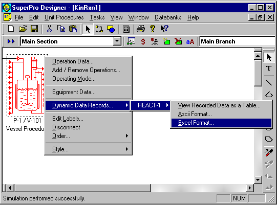
Generation of Profile data for a batch kinetic reaction.
The calculated flowrates and compositions of intermediate and output streams can be viewed by revisiting the input/output dialog windows of each stream (double click on a stream line or click with the right mouse button and select Simulation Data). In addition, a report containing information on raw material requirements, stream compositions and flowrates, as well as an overall material balance, can be generated by selecting the Tasks: Generate Stream Report (SR) option from the main menu. The resulting report can be viewed by selecting the View: Stream Report option of the main menu. The tables below display portions of the stream report. These tables were extracted from the spreadsheet version of the Stream Report, which was generated by selecting File : Export Reports to Excel. They were then edited in Excel and pasted into SuperPro as MS Excel worksheets.
OVERALL PROCESS DATA
|
Annual Operating Time |
h |
|
|
Annual Throughput |
kg MP |
|
|
Batch Throughput |
kg MP |
|
|
Plant Batch Time |
h |
|
|
Effective Plant Batch Time |
(h) |
|
|
Number of Batches Per Year |
MP = Main Product
STARTING MATERIAL REQUIREMENTS

RAW MATERIAL REQUIREMENTS ENTIRE FLOWSHEET

4.5.1 Scheduling, Equipment Utilization, and Resource Demand Graphs
SuperPro generates Operations and Equipment Gantt charts for single and multiple batches. The figure below displays a portion of the operations Gantt chart for a single batch of this example process.
The left view (spreadsheet view) displays the name, duration, start time, and end time for each activity (e.g. each operation, unit procedure, cycle, batch, etc). You can use the left view to expand or collapse the activity summaries by clicking on the + or signs in the boxes to the left of the activity names.
The right view (chart view) displays a bar for each activity in the overall process recipe. To edit the scheduling data (or any other data affecting an activity), simply right-click on a bar and a relevant command menu will appear. Selecting the uppermost entry on this menu will bring up a dialog that will allow you to edit the information associated with that particular activity bar. In fact, anything you can accomplish with the other scheduling interfaces, you can also accomplish from the Gantt chart interface. Furthermore, you can redo the M&E balances and have the Gantt Chart updated to reflect the new (calculated) scheduling settings for the recipe by clicking on the Update Chart entry in the main menu of the interface.
Operations Gantt Chart for a Single Batch.
Another way of visualizing the execution of a batch process as a function of time is through the Equipment Utilization chart (select View : Equipment Utilization Chart). The figure below displays the equipment utilization chart for two consecutive batches of this example process. Multiple bars on the same line (e.g., for R-101, R-102, NFD-101, and R-103) represent reuse (sharing) of equipment by multiple procedures. White space represents idle time. The equipment with the least idle time between consecutive batches is the time (or scheduling) bottleneck (R-102 in this case) that determines the maximum number of batches per year. Its occupancy time (approximately 54 hours) is the minimum possible time between consecutive batches (also known as Min. Effective Plant Batch Time). The actual time between consecutive batches (also known as Effective Plant Batch Time) is approximately 55 hours. The plant batch time (the time required to complete a single batch) is roughly 101 hours.
The Equipment Utilization Chart (two consecutive batches).
SuperPro also generates utilization charts for auxiliary equipment, such as clean-in-place (CIP) and steam-in-place (SIP) skids.
In addition to creating Gantt charts for equipment utilization and operations, SuperPro Designer automatically generates graphs of resource demand as a function of time for such things as heating and cooling utilities, power, labor, and raw materials. To view these graphs, select View: Resource Chart, and then choose the desired resource from the drop-down menu. The figure below displays the labor demand graph for four consecutive batches. Note that for short periods of time there is a need for up to seven operators. If this exceeds the actual number of operators available, then certain operations will need to be delayed to accommodate the labor constraint.
SuperPro is equipped with powerful throughput analysis and debottlenecking capabilities. The objective of these features is to allow the user to quickly and easily analyze the capacity and time utilization of each piece of equipment, and to identify opportunities for increasing throughput with the minimum possible capital investment. For a detailed throughput analysis example (based on this process), please see Chapter 6 or search for Debottlenecking in the Help Facility.
The Labor Demand Chart (four consecutive batches).
Below are the key results of cost analysis for a plant producing 35,200 kg of this intermediate per year. The table below gives an overview of the total economic impact of the plant, including the total capital investment, yearly revenues, and rate of return. This table was extracted from the spreadsheet version of the Economic Evaluation Report (EER). The full EER can be generated by selecting Tasks: Generate Economic Evaluation Report (EER) from the main menu. The resulting report can be viewed by selecting the View: Economic Evaluation Report option of the main menu.
Executive Summary:
The next two tables provide breakdowns of the annual operating and raw materials costs. They were extracted from the spreadsheet version of the Itemized Cost Report (ICR). The full ICR can be generated by selecting Tasks: Generate Itemized Cost Report (ICR) from the main menu. The resulting report can be viewed by selecting the View: Itemized Cost Report option of the main menu. The ICR enables the user to readily identify the cost sensitive sections of a flowsheet the economic hot-spots. For instance, a quick look at the first table below reveals that 32.7% of the operating cost is associated with raw materials, especially quinaldine (see the second table for the raw materials cost breakdown). If a lower-priced quinaldine vendor could be found, the overall process cost would be reduced significantly. Another large cost in this example is the Equipment-Dependent expenses, which account for roughly 27% of the operating cost. Increased equipment sharing may reduce this cost but may also reduce the annual throughput. Labor and Waste Treatment/Disposal occupy the 3rd and 4th positions, respectively. Labor can be reduced through increased automation. The environmental cost can be reduced through solvent recovery, purification, and reuse.
Breakdown of Operating Costs
Breakdown of Raw Materials Costs

The above analyses show how the economic reports can be used not only for estimation of the total cost of a process, but also as a tool to optimize the process through what-if scenarios. Would it make economic sense to use two reactors instead of three? It depends on how much the throughput would decrease if two reactors were used, and how much the third reactor adds to the total cost. Would a radically modified purification scheme be better than the current scheme? It depends on what equipment, reagents, etc. would be required for the modified purification, and what the overall yield of the product would be. This type of what-if analysis is quick and easy to perform using SuperPro Designer.
SuperPro generates two different reports that provide information on the environmental impact of a process. The Emissions Report provides information on emissions of volatile organic compounds (VOCs) and other regulated compounds. The Environmental Impact Report provides information on the amount and type of waste generated by a manufacturing facility. It also provides information on the fate of a compound that enters an integrated manufacturing facility.
SuperPro Designer contains a variety of formulation, packaging, and transportation unit procedures in order to capture the cost associated with such processes.
Product formulation and packaging processes often involve formation and use of discrete entities, such as tablets, bottles, boxes, etc. The flow of such entities is represented by discrete streams, which by default are displayed in blue. For more information on discrete streams and entities, please consult the Help Facility.
This design case analyzes an industrial wastewater treatment plant and demonstrates how to track the fate of multiple chemical components (constituents) in an integrated facility. The design case file, IWWT4_0, can be found in the ExamplesIndwater subdirectory. This example is suitable for users with interest in biological wastewater treatment. Other pertinent examples that are provided with Pro-Designer include the following:
|
Subdirectory |
Description |
|
MUNWATER | |
|
UPWATER | |
|
GE |
Each of these examples has a detailed ReadMe file associated with it. You can open the ReadMe files either directly from the Start Menu or from the relevant folders in the Examples directory.
The figure on the following page displays a flowsheet that represents a simplified version of an industrial activated sludge treatment plant. The flowrate and concentration of each component of the influent stream is shown below:
|
Component |
kg/h |
g/l |
|
Water | ||
|
Glucose | ||
|
Benzene | ||
|
Biomass | ||
|
Heavy Metals |
This corresponds to a relatively small plant with an average throughput of 1 million gallons per day (MGD). Glucose represents the easily biodegradable components while benzene represents the recalcitrant (not easily biodegradable) and volatile components.
Please visit the component registration dialog (select Tasks Register Components & Mixtures Pure Components), to view the physical and environmental properties of the various components. Some of the environmental properties of Glucose are shown in the table following the process flowsheet.
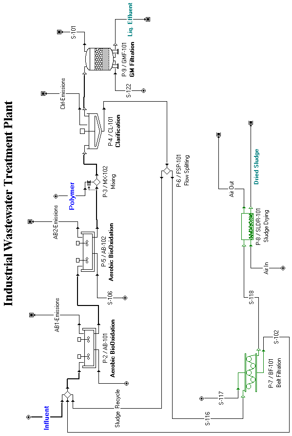
Selected Environmental Properties of Glucose:

Please note that the above values are displayed when you select the Glucose component by clicking on its line number (# 5) on the left hand side of the Registered Components table (see Section 2.5.3 for information on the Registered Components table), then click on the Properties button, and then click on the Aqueous tab. Values for such properties are available in the component database for many components. Whenever you enter a new component, you should visit its Properties dialog box to enter appropriate values for the important properties. Note that these values, along with the stream compositions, are used to calculate the lumped environmental stream properties (BOD, COD, TKN, TSS, etc.).
The influent stream is combined with the sludge return stream (Sludge Recycle) and is sent to a sequence of two aeration basins (AB-101 and AB-102) for biological oxidation of the organic material. Each aeration basin operates at an average hydraulic residence time of 6 hours and an average sludge residence time of 17.2 hours. A surface aeration system is used to maintain a minimum dissolved oxygen (DO) concentration of 2 mg/l. A clarifier (CL-101) is used to remove the biomass and thicken it to around 10 g/L solids content. The liquid effluent from the clarifier is further treated using a granular media filter (GMF-101) to remove any remaining particulate components. The withdrawn sludge (S-116) is concentrated to a 15% (wt/wt) solids content using a belt filter press (BF-101). The removed water (S-102), which contains small amounts of biomass and dissolved solids, is sent back to the aeration basin. The concentrated sludge stream is dewatered to a final solids concentration of 35% (wt/wt) using a sludge dryer (SLD-101).
At this point, please visit the interface dialogs of the various operations to check the specified parameter values. The bioconversion reaction parameters are explained in detail later in this section.
Flowsheet Sections
A flowsheet section is a group of unit procedures that have something in common. For instance, the flowsheet of this example has been divided into two sections: 1) BioOxidation and 2) Sludge Treatment. All the procedures of the Sludge Treatment section are displayed in green.
Stoichiometry and Kinetics of Biotransformations
You may view the stoichiometry and kinetics of the various reactions by visiting the reaction dialog window of the aeration basin (see figure below). As can be seen, the model offers great flexibility in specifying the kinetics of a bioreaction. A bioreaction operation (e.g., aerobic bio-oxidation) can handle any number of such reactions. Make sure you look at the MUNWATER example if you wish to distinguish between autotrophic and heterotrophic biomass and its impact on oxidation and nitrification / denitrification reactions.
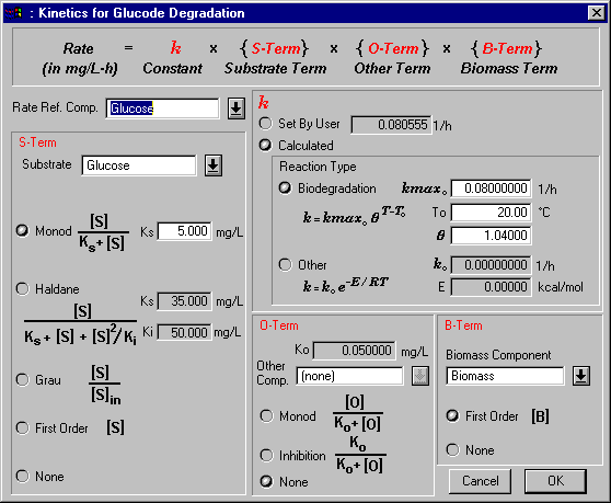
The Kinetics dialog of the Reactions tab of Aerobic BioOxidation.
The stoichiometry and kinetics of the bioconversion reactions of this example are described below. Negative coefficients are used for reactants and positive coefficients for products.
a. Glucose degradation - stoichiometry on a mass basis
Glucose ===> Biomass + H2O + CO2
-1 g 0.4 g 0.3 g 0.3 g
For those of you who are used to thinking in terms of yield coefficients, the above stoichiometry is equivalent to the following yield coefficient.
Y = 0.4 mg Biomass / mg Glucose
Note that in Pro-Designer the user never specifies yield coefficients since that information can be extracted from the reaction stoichiometry.
kmaxo = 0.08 1/h at T = 20 deg C
theta = 1.04 (to account for the impact of temperature variations).
Ks = 5 mg Glucose/ L
Note that we express the kinetic constants in terms of Glucose concentration and not BOD5 because BOD5 is not a component in Pro-Designer but a stream property. We treat BOD5 as a stream property and not as a component because many different components (e.g., Glucose, Benzene, etc.) may contribute to BOD5.
b. Benzene degradation - stoichiometry is on a mass basis
Benzene ===> Biomass + H2O + CO2
-1 g 0.3 g 0.4g 0.3 g
kmaxo = 0.019 1/h at T = 20 deg C
theta = 1.04 (to account for the impact of temperature variations).
Ks = 13.571 mg Benzene / L
c. Biomass decay
Biomass ===> DeadBiomass
-1 g 1 g
k = 0.005 1/h
Note that in Pro-Designer biomass decay is handled through a separate reaction. In other words, you do not specify a decay coefficient but instead you specify a decay reaction with its own kinetic constants. This is a richer representation compared to the traditional way because it enables the user to distinguish between active and inert biomass.
In the above reactions we ignored the consumption of oxygen and nitrogen for the sake of simplicity. If you wish to consider it, simply modify the stochiometry of the reactions and make sure that those components are available in the feed streams of the reactors.
VOC Emissions
Volatile organic compounds (VOCs) in influent streams tend to volatilize from open tanks and end up in the atmosphere. Current US EPA regulations limit VOC emissions from treatment plants to no more than 25 tons per year (Van Durme, Capping Air Emissions from Wastewater, Pollution Engineering, pp. 66-71, Sept. 1993). Pro-Designer can be used to predict VOC emissions using models that are accepted by the EPA.
In this example, emissions occur from the two aeration basins and the clarifier. Please double-click on the emission streams to see the amount of benzene that is emitted. Around 17.4% of the total incoming benzene is emitted from the first aeration basin. A much smaller amount (around 0.04% of the total incoming) is emitted from the second aeration basin and essentially none is emitted from the clarifier.
Sorption on Biomass (Sludge)
In activated sludge plants, certain compounds (e.g., heavy metals) adsorb on biomass and follow its path. In the current version of Pro-Designer, you can account for that by specifying the sorption (%) for each component that adsorbs on biomass through the Sorption tab (see figure below) of the biological reaction operations. A sorption model based on the log(Octanol/Water) partition will become available in a future release of the software.
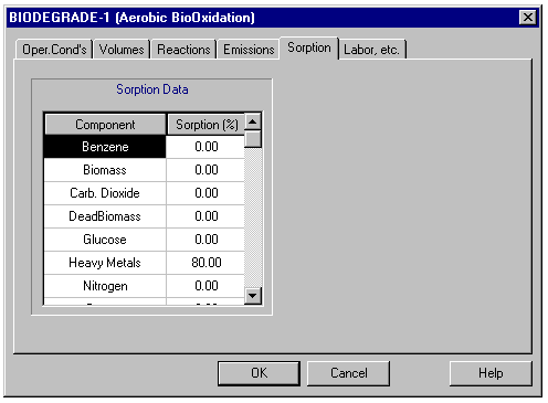
The Sorption tab of Aerobic BioOxidation.
For the sorption specifications to have an impact, you also need to identify the Primary Biomass component through the component registration dialog (select Tasks Register Components and Mixtures Pure Components). If you use more than one biomass component (e.g., heterotrophic, autotrophic, etc. as in the MUNWATER example), you should identify the heterotrophic bacteria (the most abundant) as your primary biomass.
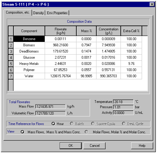
Dialog of an intermediate stream.
In a stream, the percentage of a component that is not associated with primary biomass is displayed on the stream dialog (see figure above) with the Extra-Cell % variable. In the above case, 9.76% of the total amount of Heavy Metals is extracellular (in solution) and consequently 90.24% is associated with primary biomass. This information is utilized in the material balances of separation operations. For instance, if the removal percentage of the primary biomass in a clarifier is 98%, then 98% of a sorbed component will follow the primary biomass component. Please visit the Liquid Effluent and Dried Sludge streams to see how the Heavy Metals are distributed between the two output streams.
The calculated flowrates and compositions of intermediate and output streams can be viewed by revisiting the input/output dialog windows of each stream (double click on a stream line or click with the right mouse button and select Simulation Data).
Clicking on the Env. Properties tab of a stream dialog will bring up the window shown below. This dialog window displays the compositions and flowrates of the traditional environmental stream properties (e.g., BOD, COD, TOC, TSS, etc.). The values of these properties are calculated based on the chemical composition of the stream and the contributions of the various stream components to these properties.
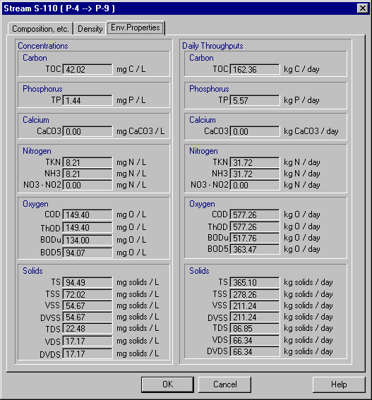
Environmental and Aqueous Stream Properties of stream S-110
Note: Information about water hardness expressed in CaCO3 is used in water purification processes for sizing Ion Exchange columns and characterizing the purity of water.
To view the flowrates and compositions of every stream on the flowsheet, you can generate the Stream Report by selecting Tasks/Generate Stream Report and then view it by selecting View/Stream Report
You may also want to look at the environmental impact assessment report (EIR), which contains information on the amount and type of waste that is generated by a manufacturing or waste treatment facility. The EIR also displays the compositions and flowrates of the traditional environmental stream properties (e.g., BOD, COD, TOC, TSS, etc.) for all the input and output streams of a process.
Before looking at the cost analysis and economic evaluation reports, it is useful to visit the Input/Output Stream Classification dialog window by selecting Tasks/Revenue, Raw Material and Waste Streams Please note that the Influent stream has been classified as a Revenue stream with a unit processing cost of $0.008/kg (or $80/m3). In other words, we assume that this plant will charge $80/m3 to the waste generators that use this facility to treat their wastewater. Please also note the unit cost of treatment/disposal that has been assigned to the various output streams.
The table below provides a breakdown of the annual operating cost. The equipment-dependent cost is the most important item even when depreciation is ignored. Depreciation can be ignored for very old plants or for plants that were built with public funding. The equipment-dependent cost includes Depreciation, Maintenance, Insurance, Local Taxes, and Factory Expense. To estimate the labor cost, it was assumed that a total of 5 operators (3 in the BioOxidation section and 2 in the Sludge Treatment section) are required to run the plant on a 24-hour basis. The unit labor cost was assumed to be $18/hour. Depending on plant location, this cost may require adjustment. The sludge disposal cost was assumed to be $50/ton. Again this may vary considerably depending on plant location.
|
Including Depreciation |
Excluding Depreciation |
||||
|
Cost Item |
$/Year |
% |
$/Year |
% |
|
|
Raw Materials |
294,000 |
294,000 | |||
|
Labor-Dependent |
414,000 |
414,000 | |||
|
Equipment-Dependent |
6,005,000 |
2,998,000 | |||
|
Laboratory/QC/QA |
62,000 |
62,000 | |||
|
Waste Trt/Disp |
1,065,000 |
1,065,000 | |||
|
Utilities |
5,000 |
5,000 | |||
|
Total |
7,845,000 |
4,838,000 | |||
To eliminate the cost of depreciation, the value of 'Portion of Purchase Cost Already Depreciated' for all the equipment items was set to 100%. The above variable is displayed on the Adjustments tab of the Equipment Data dialog of each unit procedure (right click on a procedure icon and select Equipment Data). The material for the above table was extracted from the itemized cost report (ICR) of the base case and the case that excluded depreciation.
If we had to build a plant of this size, the capital investment would be around $33.4 million. Other relevant economic results for this case appear below.
Including Depreciation:
|
TOTAL CAPITAL INVESTMENT |
33,406,000 |
$ |
|
OPERATING COST |
7,845,000 |
$/year |
|
PROCESSING RATE |
1,247,389,387 |
kg/year of Influent |
|
UNIT PROCESSING COST |
$/MT of Influent |
|
|
TOTAL REVENUES |
9,979,000 |
$/year |
|
GROSS MARGIN |
% |
|
|
RETURN ON INVESTMENT |
% |
|
|
PAYBACK TIME |
years |
Excluding Depreciation:
|
TOTAL CAPITAL INVESTMENT |
33,406,000 |
$ |
|
OPERATING COST |
4,838,000 |
$/year |
|
PROCESSING RATE |
1,247,389,387 |
kg/year of Influent |
|
UNIT PROCESSING COST |
$/MT of Influent |
|
|
TOTAL REVENUES |
9,979,000 |
$/year |
|
GROSS MARGIN |
% |
|
|
RETURN ON INVESTMENT |
% |
|
|
PAYBACK TIME |
years |
The detailed results of the economic evaluation can be produced by selecting Tasks Generate Economic Evaluation Report. To view the report, you will need to select View Economic Evaluation Report. Note that several multipliers are used to estimate the capital investment of a treatment plant and perform its cost analysis and economic evaluation. Please read the first example of this chapter for more information on how to access and modify those multipliers. Many of the current default multipliers in Pro-Designer are more appropriate for chemical manufacturing plants than wastewater treatment plants. Future versions of Pro-Designer will be provided with setting files that will include application specific multipliers. Presently, you may do something equivalent by creating a template file using your own validated multipliers. The IWWT4_0 file used for this example is a good starting point.
This example can be used as a good starting point for modeling your own wastewater treatment plants. You may add more components and/or unit procedures to this flowsheet in order to better approximate your own processes. For instance, you may add O2, NH3, and PO4, and introduce appropriate reactions for tracking the consumption and generation of those compounds. The example on municipal wastewater treatment (directory MUNWATER) provides information on modeling of nitrogen removal.
Warning! As you increase the number of components, reactions, process steps, and recycle loops, Pro-Designer will take longer to converge. Consequently, you are strongly advised to increase the complexity of your flowsheets in small steps so that you can be in a position to readily identify the changes that really slow down the convergence. For instance, reactions with very different reaction rates specified in a single unit procedure slow down the calculations considerably and may even cause convergence to fail. In such situations, it may be better to simplify your model by ignoring a slow reaction, at least at the early stages of analysis. Similarly, if you have a very fast reaction, you may want to model it using a generic reaction box (in which you specify the stoichiometry and the extent of conversion) and assume 100% conversion.
Commonly Asked Questions. Almost all new users that attempt to model biological wastewater treatment processes using Pro-Designer ask the following question:
Very often we design and operate wastewater treatment processes based on overall stream properties such as BOD, COD, TKN, SS, etc. We have no information on individual chemicals (constituents) in influent and effluent streams. Since Pro-Designer performs material balances on constituents, how can we use it to design processes based on traditional stream properties such as BOD, COD, etc.?
Answers to this and other questions can be found in the Q&A file (a hypertext type of file) that is provided with the software. For this particular question, click on Components and look at the first Q&A. The municipal wastewater treatment example (directory MUNWATER) provides additional information related to the above question.
The annual (or campaign) throughput of a batch manufacturing facility is equal to batch throughput times the number of batches that can be processed per year. Therefore, we can increase annual throughput by increasing the batch throughput or the number of batches per year or both at the same time.
![]()
In our effort to increase annual throughput we run into bottlenecks that are either equipment or resource (e.g., utilities, labor, demand for raw materials) related.
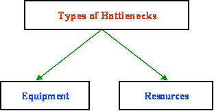
The equipment or resource that limits the number of batches per year is the Scheduling or Time Bottleneck. The equipment or resource that limits the batch throughput (amount of material processed per batch) is the Size or Throughput bottleneck. In continuous plants, we only have throughput bottlenecks.
Please note that for a batch plant the Batch Throughput and the Number of Batches per Year are interdependent. More specifically, as the batch throughput is increased (operating closer to the maximum), the cycle time of most procedures will increase resulting in longer effective plant batch times and fewer batches per year. Consequently, the maximum annual plant throughput cannot be simply set equal to the maximum batch throughput times the maximum number of batches per year. Instead, it should be calculated in an iterative way by gradually increasing the batch throughput and letting SuperPro calculate the corresponding maximum number of batches.
6.1.1 Identifying Equipment Time (Scheduling) Bottlenecks
Information on the equipment scheduling bottleneck is provided on the Recipe Scheduling Information dialog (see Chapter 2). The same information can be visualized graphically on the Equipment Utilization chart. The scheduling (or time) equipment bottleneck is the piece of equipment that has the longest cycle (occupancy) time. This piece of equipment determines the minimum time between consecutive batches and consequently the maximum number of batches per year. For equipment items that are shared by multiple procedures, their occupation time is set equal to the time interval between the start of the first procedure that is hosted by the equipment to the end of the last procedure that is hosted by the same equipment. Please note that resources also can become time bottlenecks (see section on resource bottlenecks below).
6.1.2 Identifying Equipment Size (Throughput) Bottlenecks
The Equipment Size (Throughput) bottleneck can be identified by considering the Capacity and Time utilization of each equipment item.
This variable represents the equipment capacity utilized during a certain procedure. For instance, if a piece of equipment that can process up to 100 kg/h of a certain material it is operated at a rate of 80 kg/h, its equipment capacity utilization will be 80%. If a piece of equipment is of vessel type, its capacity utilization can be defined based on the ratio of actual and maximum liquid levels for a certain operation. The figure below illustrates this in detail. The Capacity Utilization for a unit procedure is calculated by selecting the maximum capacity utilization among all operations of that procedure.

This variable represents the percent of plant operating time that a certain piece of equipment is occupied. For plants operating in batch mode, equipment uptime can be defined as follows:

Effective Plant Batch Time is the time interval between consecutive batches. If a piece of equipment is used by multiple procedures (in a batch plant), the equipment uptime accounts for the overall (of all procedures) utilization in time.
Many procedures have uptimes (as well as cycle times) that are proportional to the amount of material processed per cycle. For example, if you have a filtration procedure in which the volume of material that needs to be filtered is doubled, the filter uptime will double (assuming that the filtrate flux remains the same). Equipment items of this type usually operate at 100% capacity utilization and changes in their throughput amount only affect their uptime. This is an important point to understand just because a piece of equipment is listed at 100% Capacity Utilization does not necessarily make it a throughput bottleneck. In the filtration example, the equipment can simply be run for twice the amount of time, as long as the total filtration time does not exceed the effective batch time.
Combined Utilization of a procedure is simply its Equipment Capacity Utilization times its Equipment Uptime. To have a Combined Utilization of 100%, the procedures equipment would have to be run at maximum capacity and its cycle time would have to be the same as the effective plant batch time.
The procedure with the highest Combined Utilization % will generally be the throughput (size) bottleneck for the process. This will always be the case for unit procedures which have cycle times proportional to their throughput (whether or not a unit procedures cycle time is proportional to its throughput is noted in the Throughput Analysis Report tables). However, in some cases where the cycle time is not proportional to throughput, the unit procedure with the highest Combined Utilization will not necessary be the throughput (size) bottleneck. This can occur when particular unit procedures cannot run 100% of the time. For instance, if the plants effective batch time is 100 hours, and a series of reactions in a particular vessel takes 60 hours, you will only be able to use that vessel 60% of the time. In some cases, you may be able to run multiple cycles (and even partial cycles) to increase your equipment uptime, but in many processes (such as pharmaceuticals) this may not be an option.
A better way of identifying throughput (size) bottlenecks is by calculating the Potential Maximum Throughput (PMT) of each procedure. For procedures with cycle times proportional to their throughputs (e.g., filtration, centrifugation, etc.), the PMT is calculated by assuming 100% equipment capacity utilization and 100% uptime. For procedures whose cycle times are not proportional to their throughputs (e.g., vessel procedures, chromatography, etc.), their PMTs are calculated under Conservative, Realistic, and Theoretical assumptions for their uptimes (see figure below). The Equipment Capacity utilization is assumed to be 100% in all the cases.

In the Conservative case, the Equipment Uptime is kept the same as its current uptime.
In the Realistic case, the Equipment Uptime is set to correspond to the highest number of complete cycles that can be performed in that piece of equipment within the time window of the effective plant batch time.
In the Theoretical case, the Equipment Uptime is assumed to be at 100%. This would require mixing of partial lots of product, which may not be an option in many processes.
The objective is to identify the TRUE size (throughput) bottleneck based on the realistic scenario. The conservative scenario corresponds to the case where we operate all the equipment items at 100% capacity utilization without making any changes in the number of cycles per batch. Batch plants that are dedicated to manufacturing of a single product should be designed with equipment capacity utilization and uptime of close to 100% for all equipment items. For multi-product batch plants this is not feasible. In such cases, the above methodology can be applied to maximize the plant throughput for each separate product by identifying the appropriate capacity utilization and uptime for each procedure/equipment.
6.1.3 Resource Bottlenecks
Resources can become size (throughput) and time (scheduling) bottlenecks when their average or instantaneous demand exceeds their average or instantaneous capacity, respectively. For instance, the figure below shows the demand for labor as a function of time for three consecutive batches of a process. For short periods of time, there is a need for up to eight operators. If seven (red line) is the maximum number of operators available at any time, then certain operations will have to be delayed to accommodate that constraint. That delay of operations may increase the effective plant batch time and reduce the maximum number of batches per year and therefore become the new time bottleneck. The current version of Pro-Designer does not identify resource time bottlenecks. However, it calculates and displays the demand for any resource (e.g., raw materials, heating/cooling utilities, power, and labor) and enables the user to visualize and interactively eliminate potential resource bottlenecks. Future versions of the software will enable the user to specify maximum capacity values and the program will automatically delay certain operations in order to meet those constraints.
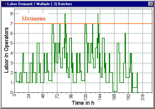
The first table below displays information on the current annual and batch throughput, the plant batch time, the number of batches per year, and the time bottleneck equipment (NFD-101 in this case).
OVERALL PROCESS DATA
Annual Operating Time = 7883.68 h
Annual Throughput = 28463.53 kg MP
Batch Throughput = 171.47 kg MP
Plant Batch Time = 81.60 h
Number of Batches Per Year = 166
Time Bottleneck Equipment = NFD-101
MP = Main Product = Total Flow in Final Product
The second table (see below) displays information on Equipment Capacity Utilization, Equipment Uptime, and Combined Utilization for all the procedures of a flowsheet. The procedure with the highest Combined Utilization (P-11 in this case) is considered the Throughput (Size) Bottleneck based on this approach. Please note that this may not be the true bottleneck under real world conditions. Equipment items that are in Design Mode do not appear on these tables because their size is calculated by the program to meet the current processing demand.
EQUIPMENT CAPACITY UTILIZATION AND UPTIME (Entire Flowsheet)
Equipment Procedure Capacity Equipment Combined
Tag Name Utilization Uptime Utilization
(%) (%) (%)
R-101 P-1 53.18 43.77 23.28
P-7 61.62 43.77 26.97
R-102 P-3 68.22 60.24 41.09
P-9 69.69 60.24 41.98
NFD-101 P-4 100.00 37.46 37.46
P-6 100.00 37.46 37.46
P-8 100.00 37.46 37.46
P-10 100.00 37.46 37.46
P-12 100.00 37.46 37.46
R-103 P-5 57.25 46.94 26.87
P-11 99.99 46.94 46.94
TDR-101 P-13 100.00 26.26 26.26
Limiting Equipment / Procedure R-103 / P-11
The third table is a summary of potential maximum throughput (PMT) under conservative, realistic and theoretical assumptions for equipment uptime. It also identifies the bottlenecks (limiting procedure and equipment item) under each assumption. For each category, the bottleneck is the procedure with the lowest value of PMT. In this case, the same procedure (P-11 in R-103) is the conservative, realistic and theoretical size bottleneck. The bottleneck identified based on the theoretical PMT approach is always the same as the one identified by the Combined Utilization approach (previous table).
SUMMARY OF THROUGHPUT INCREASE OPTIONS (Throughput in kg MP/batch)
Equipment Procedure POTENTIAL MAXIMUM THROUGHPUT
Tag Name Conservative Realistic Theoretical
R-101 P-1 322.42 322.42 736.66
P-7 278.28 278.28 635.81
R-102 P-3 251.36 251.36 417.26
P-9 246.03 246.03 408.41
NFD-101 P-4 457.69 457.69 457.69
P-6 457.69 457.69 457.69
P-8 457.69 457.69 457.69
P-10 457.69 457.69 457.69
P-12 457.69 457.69 457.69
R-103 P-5 299.51 299.51 638.08
P-11 171.48 171.48 365.32
TDR-101 P-13 653.06 653.06 653.06
Limiting Equipment R-103 R-103 R-103
Limiting Procedure P-11 P-11 P-11
The rest of the report displays the individual potential throughput figures for each unit procedure, based on the Conservative, Realistic, and Theoretical assumptions. Furthermore, the limiting procedure and equipment bottlenecks are identified for each section of the flowsheet in their respective Section Summaries.
Procedure Name P-1 (Chlorination, Salt Formation)
Equipment Name R-101 (shared with other procedures)
Limiting Operation Separate Aqueou
Throughput Equipment Equipment Plant
Increase Capacity Uptime Throughput
Options Util.(%) (%) kg MP/batch
Conservative 100.00 43.77 322.42
Realistic 100.00 43.77 322.42
Theoretical 100.00 100.00 736.66
Current State 53.18 43.77 171.47
Cycle Time is Not Proportional to Throughput
This example is based on the Synthetic Pharmaceutical design case (SynPharm directory) that is described in Chapter 4 of this document. The goal is to produce at least 33,000 kg/year of our pharmaceutical intermediate compound in the most economical way possible by utilizing existing equipment. Here is a brief description of the design cases:
File SPhr4_0L: This process is based on lab-scale data, which has been scaled up to pilot plant production volumes. At this point all equipment is in Design Mode. In other words, the equipment capacities have not yet been defined.
File SPhr4_0a: This process was designed based on pilot plant volumes of reagents in manufacturing scale equipment. It is the same as SPhr4_0L except that the calculation mode for all equipment items has been switched to Rating. In addition, the reactors and filter are used for multiple unit procedures. Two 1000 gal reactors, one 4 m2 filter and one 10 m2 tray dryer are utilized.
File SPhr4_0b: This process is the same as SPhr4_0a, but the throughput has been scaled to 100% capacity utilization of the limiting-size reactor (R-102).
File SPhr4_0c: This process is the same as SPhr4_0b, except that THREE reactors are used in order to decrease the plants effective batch time (so that more cycles can be run per year).
File SPhr4_0d: This process is the same as SPhr4_0c except that a second filter (NFD-102) has been added.
File SPhr4_0e: This is the same as SPhr4_0d except that procedure P-11 in R-103 (and subsequent procedures) have been split into two cycles, and the batch throughput has been increased to 100% in the new capacity-limiting piece of equipment (R-102).
File SPhr4_0f: This is the same as SPhr4_0e except that the utilization of several reactors has been rearranged. Specifically, the reactors for procedures P-5 and P-7 have been switched. This allows more cycles to be run per year because the batch cycle time of reactor R-103 is decreased.
These design cases will be analyzed in greater detail later in this section. In order to save space, only certain parts of the Throughput Analysis Reports are reproduced below. To see all Throughput Analysis tables in their entirety, please open the SPhr4_0 (L, a, b, c, d, e or f) example files and create the reports as follows: click on Tasks: Generate Throughput Analysis Report. Then click on View: Throughput Analysis Report.
Interpreting the Throughput Analysis Report
The throughput analysis results for file SPhr4_0a show that Procedure P-11 in reactor R-102 is the limiting step (see table below). In other words, if we try to increase batch throughput (material processed per batch) without installing extra equipment, R-102 will become the first throughput bottleneck. The current batch size is kg of pharmaceutical intermediate. This corresponds to 32.5% capacity utilization of R-102 in Procedure P-11. If the process were scaled up to full Capacity Utilization of R-102, the throughput could be increased to 171.48 kg/batch. This is exactly what we do in file SPhr4_0b. Note - to adjust the throughput of the entire flowsheet automatically, you can go to Tasks: Adjust Plant Throughput, and then enter a scaling factor to adjust the throughput to the desired level. This adjustment can be done universally (all input streams are multiplied by the same factor) or stream-by-stream. Please remember to redo the simulation calculations after the throughput adjustment (by clicking the Solve icon, or selecting: Tasks/Solve M&E Balances).
The throughput analysis results for SPhr4_0b (please open the report and view the results) show that the effective plant batch time increases to 57.79 hours (it was 40.69 hours in SPhr4_0a). The increased batch cycle time is due to the fact that some operations in this example (such as filtration) have their cycle times specified to be proportional to flowrates. Since the total batch size was increased, the total volume of liquid that flows through the filters was increased. Thus the time required for these operations increased proportionally. The larger batch time causes the number of batches per year to decline from 194 (in SPhr4_0a) to 136. This is based on a 7920 hour maximum for the annual plant operating time. The annual operating time can be changed through the Recipe Scheduling Information dialog (select Tasks: Recipe Scheduling Information). Despite the lower number of batches per year, the increase in capacity utilization of R-102 increases the overall annual throughput of this process (recall that the annual throughput is equal to the number of batches per year times the batch throughput.) The original annual throughput was 10,810 kg, but by increasing the capacity utilization of R-102 we reach an estimated annual throughput of 23,320 kg.
EQUIPMENT CAPACITY UTILIZATION AND UPTIME (Entire Flowsheet)
Equipment Procedure Capacity Equipment Combined
Tag Name Utilization Uptime Utilization
(%) (%) (%)
R-101 P-1 17.28 65.42 11.31
P-5 18.60 65.42 12.17
P-9 22.65 65.42 14.82
R-102 P-3 22.17 58.01 12.86
P-7 20.02 58.01 11.62
P-11 32.50 58.01 18.85
NFD-101 P-4 100.00 15.82 15.82
P-6 100.00 15.82 15.82
P-8 100.00 15.82 15.82
P-10 100.00 15.82 15.82
P-12 100.00 15.82 15.82
TDR-101 P-13 100.00 11.02 11.02
Limiting Equipment / Procedure R-102 / P-11
The Equipment Capacity Utilization and Uptime table for file SPhr4_0a.
After scaling file SPhr4_0a up by roughly 3-fold, the Capacity Utilization % of the other pieces of equipment is higher as well (the lowest Capacity Utilization becomes 53.18% during P-1). At this point, other options can be considered to lower the cycle time or increase the batch size. One option is to buy more equipment so that each piece of equipment is used for fewer unit procedures. This is what is done in file SPhr4_0c. This file is identical to SPhr4_0b, except that an extra 1,000 gal reactor (for a total of three reactors) has been added. The decision to add this unit was based on a review of the multiple batch Equipment Utilization Chart for SPhr4_0b (see below.) A quick look at this chart reveals that R-101 is the current scheduling bottleneck. If a third reactor is added, the batch cycle times for R-101 and R-102 can be reduced because fewer unit procedures will take place in each reactor. After adding the third reactor (in SPhr4_0c), the effective batch time decreases to 47.3 hours, and the number of cycles per year is increased to 166. This allows the annual throughput to increase to 28,464 kg/yr. It should be noted that the purchase of an additional reactor significantly increases the overall cost of the project. In fact, despite the increased throughput possible under this setup, the Internal Rate of Return (IRR) for this process actually decreases from 56.0% to 50.1% (The IRR is listed in the Economic Evaluation Report and the Executive Summary). In some situations, a decrease in IRR caused by buying more equipment could be much greater than the decrease calculated for this particular example. Thus, although adding extra equipment units or buying larger pieces of equipment are obvious methods to increase throughput, they sometimes have a negative effect on the overall economics of the process (other times the increase in throughput more than compensates for the increased capital expenditure). This is why the economic reports should be used in conjunction with the Throughput Analysis Report when determining the best setup for your process.
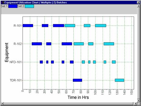
The multiple-batch Equipment Utilization Chart for SPhr4_0b
After the third reactor is added (file SPhr4_0c) another Equipment Utilization Chart is produced (see below). This chart shows that the new equipment bottleneck is the filter NFD-101.
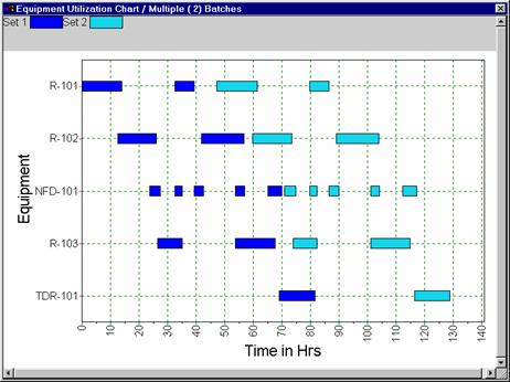
The multiple-batch Equipment Utilization Chart for SPhr4_0c
Since we have not yet reached our target of 33,000 kg/year, we must increase throughput again. One way to do this is to purchase a second filter. This will further decrease the effective plant batch time and therefore increase the number of batches produced per year. The use of a second filter is incorporated in file SPhr4_0d, and the new multi-batch equipment utilization chart is displayed below. With this change, the number of batches per year increases from 166 to174, and the new annual throughput goes from 28,464 kg/yr to 29,836 kg/yr. Although the addition of the second filter does not increase the annual throughput greatly, it is relatively inexpensive and it will allow us to make several additional changes that will increase both the annual throughput and the IRR.
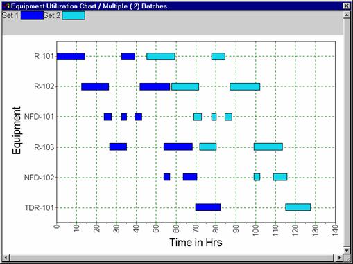
The multiple-batch Equipment Utilization Chart for SPhr4_0d
After adding another filter, our options for increasing throughput become more limited. Addition of more equipment will not decrease the effective batch time very much (unless 3 more reactors are added so that each unit procedure has its own dedicated piece of equipment.) However, if we look at the Throughput Analysis Report for SPhr4_0d (see below), it becomes apparent that only one unit procedure (P-11 in R-103) uses its full equipment capacity. Note recall that the filters and dryer listed below are not really at full capacity because an increase in throughput would simply increase their cycle times and uptime, as opposed to overfilling them. If we split the batch in half for procedure P-11, we will no longer be constrained by the capacity of R-103. As a result, we will be able to increase the batch throughput in all other pieces of equipment. This is what is done in file SPhr4_0e; procedure P-11 (and subsequent procedures) are split into 2 cycles, and the batch throughput is increased to the point where the new capacity bottleneck (P-9 in R-102) is at maximum utilization. Procedure P-10 is also switched from NFD-102 to NFD-101. When this is done, the total number of batches per year is decreased from 174 to 135 because the equipment uptime for R-103 is increased. However, the batch throughput is increased from 171.47 kg/batch to 246.05 k/batch. As a result, the annual throughput increases from 29,836 kg/yr to 33,217 kg/yr. This meets our goal of producing 33,000 kg/year of our product. However, one other simple change can be made which will further increase throughput, as well as increase the projects return on investment. Please refer to the multi-batch Equipment Utilization Chart for file SPhr4_0e on the next page.
EQUIPMENT CAPACITY UTILIZATION AND UPTIME (Entire Flowsheet)
Equipment Procedure Capacity Equipment Combined
Tag Name Utilization Uptime Utilization
(%) (%) (%)
R-101 P-1 53.18 45.75 24.33
P-7 61.62 45.75 28.19
R-102 P-3 68.22 62.97 42.95
P-9 69.69 62.97 43.88
NFD-101 P-4 100.00 21.55 21.55
P-6 100.00 21.55 21.55
P-8 100.00 21.55 21.55
R-103 P-5 57.25 47.51 27.20
P-11 99.99 47.51 47.51
NFD-102 P-10 100.00 17.65 17.65
P-12 100.00 17.65 17.65
TDR-101 P-13 100.00 27.45 27.45
Limiting Equipment / Procedure R-103 / P-11
The Equipment Capacity Utilization and Uptime table for SPhr4_0d
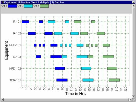
The multiple-batch Equipment Utilization Chart for SPhr4_0e
The SPhr4_0e Equipment Utilization Chart above reveals that there is one other easy way to increase throughput for this process: rearrange the reactor utilization sequence. If the second procedure in R-101 (P-7) is switched to R-103, and the first procedure in R-103 (P-5) is switched to R-101, the batch cycle time of each is shortened. This allows the effective batch time to be cut to 54.86 hours, which increases the number of batches per year to 143 and increases the annual throughput to 35,185 kg. Of course, the calculated values for annual throughput, IRR, etc., are only as good as the data that was used to produce them. However, the trends in IRR, annual throughput, etc., are likely to be correct if you have modeled your process correctly. For instance, it is easy to understand that by going from example SPhr4_0e to SPhr4_0f you will have a better IRR since you are increasing your annual throughput simply by changing your procedure scheduling (and without buying additional equipment, etc.)
Even after the scheduling of unit procedures in these three reactors has been optimized, there will be gaps between their uptime periods (none of the equipment is running 100% of the time). This will be typical of most batch processes. As the unit procedures in this example (SPhr4_0f) are currently configured, the only way to have constant utilization of any given piece of equipment would be to have fractional batches during a given cycle. For example, reactor R-101 has an Uptime of 61.74% (see table below). Thus in order to have constant utilization of this reactor, roughly 1.62 batches would have to be produced in R-102 during each plant batch cycle. Mixing of different lots can be highly undesirable (or even strictly prohibited) in many processes, especially production of pharmaceuticals. If mixing of different material lots was allowed, the maximum possible throughput during the current effective batch time (without installing additional equipment) would be 398.52 kg of our synthetic pharmaceutical intermediate, which corresponds to 100% Combined Utilization of the throughput-limiting piece of equipment (P-9/R-102).
EQUIPMENT CAPACITY UTILIZATION AND UPTIME (Entire Flowsheet)
Equipment Procedure Capacity Equipment Combined
Tag Name Utilization Uptime Utilization
(%) (%) (%)
R-101 P-1 76.29 48.75 37.19
P-5 82.15 48.75 40.05
R-102 P-3 97.89 61.74 60.44
P-9 100.00 61.74 61.74
NFD-101 P-4 100.00 51.92 51.92
P-6 100.00 51.92 51.92
P-8 100.00 51.92 51.92
P-10 100.00 51.92 51.92
R-103 P-7 88.42 58.94 52.12
P-11 71.74 58.94 42.28
NFD-102 P-12 100.00 38.72 38.72
TDR-101 P-13 100.00 43.63 43.63
Limiting Equipment / Procedure R-102 / P-9
The Equipment Capacity Utilization and Uptime table for SPhr4_0f
Following the Equipment Capacity Utilization and Uptime table in the Throughput Analysis Report is the Summary of Throughput Increase Options table (see below). This table lists the Potential Maximum Throughput (PMT) for each unit procedure under the Conservative, Realistic, and Theoretical assumptions defined previously (please see section 6.1). It also identifies the bottlenecks (limiting procedure and equipment item) under each assumption. The highest potential throughput (using the current equipment configuration) is represented by the lowest value in the column of this table that corresponds to the assumption you used (Conservative, Realistic, or Theoretical). For instance, if you are interested in the maximum possible throughput under the Conservative assumption, you should look for the lowest value under the Conservative column. This value is 246.05 kg, which is listed next to procedure P-9 in R-102. (A batch throughput of 246.05 kg is also the current throughput, as we can see from the very first table in the Throughput Analysis Report see below). Similarly, the maximum possible throughputs under the Realistic and Conservative assumptions are 246.05 kg and 398.53 kg, respectively.
SUMMARY OF THROUGHPUT INCREASE OPTIONS (Throughput in kg MP/batch)
Equipment Procedure POTENTIAL MAXIMUM THROUGHPUT
Tag Name Conservative Realistic Theoretical
R-101 P-1 322.53 322.53 661.53
P-5 299.51 299.51 614.33
R-102 P-3 251.36 251.36 407.12
P-9 246.05 246.05 398.52
NFD-101 P-4 473.89 473.89 473.89
P-6 473.89 473.89 473.89
P-8 473.89 473.89 473.89
P-10 473.89 473.89 473.89
R-103 P-7 278.28 278.28 472.12
P-11 342.99 342.99 581.91
NFD-102 P-12 635.46 635.46 635.46
TDR-101 P-13 563.92 563.92 563.92
Limiting Equipment R-102 R-102 R-102
Limiting Procedure P-9 P-9 P-9
The Summary of Throughput Increase Options table for SPhr4_0f.spf.
OVERALL PROCESS DATA
Annual Operating Time = 7890.60 h
Annual Throughput = 35185.07 kg MP
Batch Throughput = 246.05 kg MP
Plant Batch Time = 100.79 h
Number of Batches Per Year = 143
Time Bottleneck Equipment = R-102
MP = Main Product = Total Flow in Final Product
Additional tables in the Throughput Analysis Report display the individual potential throughput figures for each unit procedure, based on the Conservative, Realistic, and Theoretical assumptions. Furthermore, the limiting procedure and equipment bottlenecks are identified for each section of the flowsheet in their respective Section Summaries.
One of the fundamental differences between Version 3 and Version 4 of SuperPro Designer is the use of Unit Procedures. A Unit Procedure is a set of operations that take place sequentially in a piece of equipment. For instance, a Unit Procedure that takes place in a chemical reactor may include: Charge Material A, Heat, Charge Material B, Agitate, React, Charge Extraction Solvent, Extract (Phase Split), Discharge Bottom Phase, Transfer Out Top Phase, etc. This set of operations is displayed on the process flow diagram (PFD) with a single reactor icon. The operations within a Unit Procedure may take place sequentially, simultaneously, or relative to a given starting point.
Please note the change in terminology and structure between Version 3 and Version 4 of SuperPro Designer: in Version 3, a Unit Operation such as a reaction or filtration was represented by a single icon on the flowsheet, whereas in Version 4 multiple Operations can take place within each Unit Procedure. This change allows for greater flexibility and specification of details within each operation. For instance, the Nutsche Filtration from Version 3 can now been broken down into: Filtration, Wash Cake, Dry Cake, Transfer Out, and other operations if desired. The usage of Unit Procedures also simplifies complex PFDs by allowing many operations which occur sequentially in the same piece of equipment to be represented by one icon on the flowsheet. For instance, a sequence such as: React, Extract, Distill, and Crystallize which all occur in Reactor-101 can now be represented as one icon.
In order to better visualize the scheduling aspects of processes, two new Gantt charts have been added to replace the original Gantt chart in Version 3. One of the new Gantt charts displays the execution of the Unit Procedures as a function of time. Double-clicking on the name of a Unit Procedure expands its view to display the list of all operations that are included in that Unit Procedure. The second chart displays the utilization of each piece of equipment as a function of time. Both charts are capable of displaying single and multiple batches. To view the Gantt charts, click on Tasks: Gantt Charts, and then choose from the list of options. For more information on the Gantt chart features, refer back to chapters 3.3 and 4.5, or look up Gantt using the SuperPro Help facility.
In addition to the new Gantt charts, demand for various resources can now be tracked as a function of time. Resources include all heating and cooling utilities, power, labor, and all raw materials (pure components as well as stock mixtures.) This will enable the user to identify and eliminate resource bottlenecks. It will also facilitate sizing and design of batch utilities (e.g. steam, clean steam, WFI, etc.). To see the resource charts, click on View: Resource Chart, and choose from the list of options.
The Throughput Analysis capabilities of SuperPro Designer have also been greatly enhanced. To find out more about throughput analysis and debottlenecking, please refer to chapter 6.
Improvements have been made (in collaboration with Amersham-Pharmacia Biotech) to the chromatography models, including the addition of an expanded bed adsorption (EBA) chromatography column.
Volatile Organic Compound (VOC) emission models have been added to batch operations such as Charge, Heat, Purge, Evacuate, Gas Sweep, React, Vaporize, etc. The user has the option of specifying whether these emission calculations should affect the material balances.
An important new Unit Procedure in Version 4.0 is the Vessel Procedure. This procedure is designed to be highly flexible. Vessel Procedures may take place in reactors or various types of fermentors. The operations that are available in the Vessel Procedure include: Charge, Transfer In, Transfer Out, Heat, Cool, React (three options Stoichiometric, Kinetic, and Equilibrium), Ferment (in the Fermentation Vessel Procedures), Extract/Phase Split, Vaporize/Concentrate, Distill, Crystallize, Gas Sweep, Purge/Inert, Evacuate, Pressurize, Vent, Agitate, Hold, Clean In Place (CIP), and Steam In Place (SIP). This range of operations within the Vessel Procedure offers greater potential for the user to customize the flowsheet so that it accurately reflects plant activities.
A number of major changes have been made to the underlying architecture of the SuperPro Designer software suite. Due to the magnitude of these changes, there is currently no tool available to convert Version 3 files directly to Version 4. Instead, if there is a desire to upgrade current processes to use the new version of the software, the data will have to be manually entered. The best way to do this is to generate and print out the PFD and Input Data Report using Version 3.0 and reenter the data into Version 4. If you have any difficulties, please do not hesitate to call our technical support at: (973) 622-1212 or (908) 654-0088, or email us at TechSupport@intelligen.com. Please note -- if you plan to update files in this way, do not uninstall your Version 3 software until after all of your current design files have been entered into Version 4.
To export any report in spreadsheet format, select File:Export Reports to Excel. This generates tab-delimited versions of the above files that can be opened by Excel and other speadsheets.
SuperPro Designer allows you to integrate all the drawings you have created and the results that you have generated very easily into your reports by copying and pasting objects using the clipboard.
To copy objects using the clipboard, select the elements (process steps, streams and visual objects) of the design case that you wish to include in the exported picture. If the entire flowsheet needs to be copied, you may choose Edit: Select All in order to select all elements in the currently active design case. Bring up the program where you want to include the drawings (e.g., MS-Word) and open the document that will receive the drawings. Go to the Edit menu; you have two choices:
a. Select Paste
(or alternatively, hit Ctrl+V
or Ctrl+Ins, or click
on the paste button: ![]()
b. Select Paste Special from the Edit menu. After you have chosen Edit/Paste Special the following
dialog will appear:
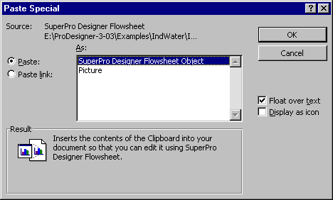
Notice that you have two decisions to make in this dialog.
The first decision refers to the nature of the pasted object as it will continue
to exist in the receiving application. Your choices are displayed in the
listbox:
(a) xxxPro Designer Flowsheet
Object, or
(b) Picture
If you select Picture, then the advantage is that most word processors will
allow you to edit that picture locally, in case you need to add to or remove
anything from it. If you select ProDesigner Flowsheet Object, then only your
copy of our Pro-Designer series software will be able to edit the contents of
the pasted picture. The second decision that you must make in this dialog is
whether you wish the pasted picture to be:
(a)
Pasted, or
(b) Paste-Linked
into the receiving document. There is a significant difference between options
(a) and (b) above. If you choose (b), the picture will be paste-linked into the
receiving document, which means that there will continue to be a live
connection (sometimes referred to as hot-connection) between the receiving
document and the source of the pasted image, the Pro-Designer design case
file. If you modify the contents of the source file, then the image in the
receiving document will change as well to reflect the most current version of
the design case. However, this behavior sometimes is not what you want. Instead
you may want to insert a frozen picture of the design case as is now, and not
have it change later. In this case you must choose (a) (i.e., simple pasting is
appropriate).
Most Windows applications (e.g., spreadsheets, word processors, etc.) allow you to insert in their document a picture (read from a file). By far the most popular graphics format in the Windows world is the so-called Windows Metafile format, or wmf format for short. It is very popular because it allows graphics to be saved and later pasted within a frame of a given size with minimal distortion of picture quality. Furthermore, several of the leading word processing and graphics applications can recognize each component in a wmf graphic and allow the graphic to be edited using their own picture editor. MS-Word, for example, has its own metafile picture editor. Therefore, you can insert a picture into MS-Word from a wmf file, resize it, edit it, and later save it again as part of the MS-Word document. SuperPro Designer allows you to export the drawing of a design case in a file with the Windows Metafile format. Heres how:
First, open (if it is not already open) the design case whose flowsheet you want to export as a wmf file (using File: Open, or Ctrl+O) and select the part of the drawing that you wish to export.
While the desired flowsheet is displayed in a workspace window, pick the File: Export Items to Metafile option; the usual Save As dialog will appear, prompting you to type the name of a file. Type in the filename that you wish to contain the description of the flowsheet in wmf format. By convention, all such files should have a .wmf extension.
After you have typed in the file name and clicked OK, the program will create the metafile-formatted description of the flowsheet. When this process is done, you can go to your favorite graphics or word processor application and import the file you have just created.
SuperPro Designer allows you to import foreign documents or
document fragments and make them part of your design case file. Using the
latest OLE technology, you can import an object copied into the clipboard from
another OLE-server application (e.g., MS-Excel,
Go to Excel and copy the spreadsheet cells that you need to display in the flowsheet. If you dont know how to select a range of cells from an Excel spreadsheet, please consult your Excel manual.
Bring up SuperPro Designer and left-click with the mouse where you would like the spreadsheet to be pasted.
Now, select Edit: Paste (or Ctrl+V
Various preferences can be specified for each design file. For instance, by clicking Edit: Flowsheet Options: Preferences: Default Styles, the user can edit the appearance defaults for Text Style, Visual Objects, Procedure Icons, Bulk Streams, Discrete Streams, Gantt charts, and various resource charts. Alternatively, these dialogs can be brought up by right-clicking on a blank portion of the screen and selecting Preferences: Default Styles. These defaults can still be overridden for individual objects, streams, etc. if desired. In addition, the user can change the default simulation convergence parameters by choosing Edit: Flowsheet Options: Convergence Parameters, or by right-clicking on a blank portion of the screen and choosing Convergence Parameters.
The throughput of a plant can be adjusted (scaled up or down) by selecting Tasks: Adjust Plant Throughput from the main menu. This brings up a dialog that allows the user to specify a scale up/down factor for all input streams of a flowsheet or for individual input streams. After a throughput adjustment, you must recalculate the material and energy balances. See chapter 2.5.6 for more information on how to perform the material and energy balances.
If several processing steps are in Rating Mode (size of equipment is specified), a scale up adjustment may result in a plant throughput that exceeds the capacity of certain equipment items. In that case, the program displays appropriate warning messages and provides instructions on how to fix the problem.
For a given batch plant of fixed equipment sizes, a scale up action usually increases the minimum effective plant batch time (the minimum possible time between consecutive batches) and decreases the maximum number of batches per year. As a consequence, there is an optimum value of batch throughput that corresponds to maximum annual throughput.
Chapter 10: Summary
We at Intelligen hope that this brief tour of the major functions of SuperPro Designer has convinced you that it is the fastest, easiest, and most cost-effective means of evaluating either continuous or batch chemical manufacturing and environmental processes. We encourage you to use the on-line help facility to explore all the features in SuperPro Designer. If you have difficulty using SuperPro, please do not hesitate to contact our tech-support office.
A New Way of Thinking. The use of SuperPro, like most other software tools, requires a new way of thinking. This is particularly important for those of you who have little or no previous experience in process simulation. Remember that with simulation we only attempt to approximate the behavior of the real world. It is impossible to completely represent the behavior of a chemical or wastewater treatment plant on the computer. Consequently, your objective should be to limit the analysis to those variables that are of interest to you from a design (if the objective is to design a new plant or retrofit an existing one) or operations (if the goal is to improve the performance of an existing plant) point of view.
For more information or to order a complete authorized copy of SuperPro Designer, mail, phone, fax, or e-mail your inquiry to the address below:
|
Politica de confidentialitate | Termeni si conditii de utilizare |

Vizualizari: 10841
Importanta: ![]()
Termeni si conditii de utilizare | Contact
© SCRIGROUP 2024 . All rights reserved