Basic Control Actions and Response of

Basic Control Actions and Response of

Control Systems

1. INTRODUCTION

An automatic controller compares the actual value of the plant output with the reference input (desired value), determines the deviation, and produces a control signal that will reduce the deviation to zero or to a small value. The manner in which the automatic controller produces the control signal is called the control action.

In this chapter we shall first discuss the basic control actions used in industrial control systems. Then we shall discuss the effects of integral and derivative control actions on the system response. We shall next consider the response of higher-order systems. Any physical system will become unstable if any of the closed-loop poles lies in the right-half s plane. To check the existence or nonexistence of such right-half plane poles, the Routh stability criterion is useful. We shall include discussions of this stability criterion in this chapter.

Many industrial automatic controllers are electronic, hydraulic, pneumatic, or their combinations. In this chapter we present principles of pneumatic controllers, hydraulic controllers, and electronic controllers.

The outline of this chapter follows: Section 5-1 has presented introductory material. Section 5-2 gives the basic control actions commonly used in industrial automatic controllers. Section 5-3 discusses the effects of integral and derivative control actions on system performance. Section 5-4 deals with higher-order systems and Section 5-5 treats Routh's stability criterion. Sections 5-6 and 5-7 discuss pneumatic controllers and hydraulic controllers, respectively. Here we introduce the principle of operation of pneumatic and hydraulic controllers and methods for generating various control actions.

Section 5-8 treats electronic controllers using operational amplifiers. Section 5-9 discusses phase lead and phase lag in sinusoidal response. Finally, in Section 5-10 we treat steady-state errors in system responses.

2 BASIC CONTROL ACTIONS

In this section we shall discuss the details of basic control actions used in industrial ana-1 log controllers. We shall begin with classifications of industrial analog controllers.

Classifications of industrial controllers. Industrial controllers may be classified according to their control actions as:

Two-position or on-off controllers

Proportional controllers

Integral controllers

Proportional-plus-integral controllers

Proportional-plus-derivative controllers

Proportional-plus-integral-plus-derivative controllers

Most industrial controllers use electricity or pressurized fluid such as oil or air as power sources. Controllers may also be classified according to the kind of power employed in the operation, such as pneumatic controllers, hydraulic controllers, or electronic controllers. What kind of controller to use must be decided based on the nature of the plant and the operating conditions, including such considerations as safety, cost, availability, reliability, accuracy, weight, and size.

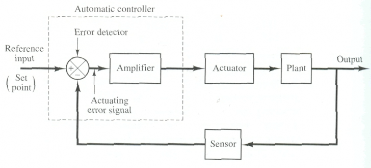
Automatic controller, actuator, and sensor (measuring element). Figure 5-11 is a block diagram of an industrial control system, which consists of an automatic controller, an actuator, a plant, and a sensor (measuring element). The controller detects the actuating error signal, which is usually at a very low power level, and amplifies it to a sufficiently high level. The output of an automatic controller is fed to an actuator, such as a pneumatic motor or valve, a hydraulic motor, or an electric motor. (The actuator is

Figure 5-1 Block diagram of an industrial control system, which consists of an automatic controller, an actuator, a plant, and a sensor (measuring element).

a power device that produces the input to the plant according to the control signal so that the output signal will approach the reference input signal.)

The sensor or measuring element is a device that converts the output variable into another suitable variable, such as a displacement, pressure, or voltage that can be used to compare the output to the reference input signal. This element is in the feedback path of the closed-loop system. The set point of the controller must be converted to a reference input with the same units as the feedback signal from the sensor or measuring element.

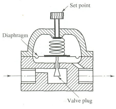
Self-operated controllers. In most industrial automatic controllers, separate units are used for the measuring element and for the actuator. In a very simple one, however, such as a self-operated controller, these elements are assembled in one unit. Self-operated controllers utilize power developed by the measuring element and are very simple and inexpensive. An example of such a self-operated controller is shown in Figure 5-2. The set point is determined by the adjustment of the spring force. The controlled pressure is measured by the diaphragm. The actuating error signal is the net force acting on the diaphragm. Its position determines the valve opening.

The operation of the self-operated controller is as follows: Suppose that the output pressure is lower than the reference pressure, as determined by the set point. Then the downward spring force is greater than the upward pressure force, resulting in a downward movement of the diaphragm. This increases the flow rate and raises the output pressure. When the upward pressure force equals the downward spring force, the valve plug stays stationary and the flow rate is constant. Conversely, if the output pressure is higher than the reference pressure, the valve opening becomes small and reduces the flow rate through the valve opening. Such a self-operated controller is widely used for water and gas pressure control.

Two-position or on-off control action. In a two-position control system, the actuating element has only two fixed positions, which are, in many cases, simply on and off .Two-position or on-off control is relatively simple and inexpensive and, for this reason, is very widely used in both industrial and domestic control systems.

Let the output signal from the controller be and the actuating error signal be e(t). In two-position control, the signal remains at either a maximum or minimum value, depending on whether the actuating error signal is positive or negative, so that

Figure 5-2 Self-operated controller.

for

for

where and are constants. The minimum value is usually either zero or - Two-position controllers are generally electrical devices, and an electric solenoid- operated valve is widely used in such controllers. Pneumatic proportional controllers with very high gains act as two-position controllers and are sometimes called pneumatic two-position controllers.

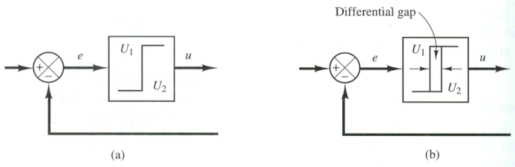
Figures 5-3 (a) and (b) show the block diagrams for two-position controllers. The range through which the actuating error signal must move before the switching occurs is called the differential gap. A differential gap is indicated in Figure 5-3(b). Such a differential gap causes the controller output to maintain its present value until the actuating error signal has moved slightly beyond the zero value. In some cases, the differential gap is a result of unintentional friction and lost motion; however, quite often it is intentionally provided in order to prevent too frequent operation of the one-off mechanism.

Consider the liquid-level control system shown in Figure 5-4(a), where the electromagnetic valve shown in Figure 5-4(b) is used for controlling the inflow rate. This valve is either open or closed. With this two-position control, the water inflow rate is either a positive constant or zero. As shown in Figure 5-5, the output signal continuously moves between the two limits required to cause the actuating element to move from one fixed

Figure 5-3 (a) Block diagram of an on-off controller; (b) block diagram of an on-off controller with differential gap.

Figure 5-4 (a) Liquid-level control system; (b) electromagnetic valve.

Figure 5-5 Level versus t curve for the system shown in Figure 5-4(a).

position to the other. Notice that the output curve follows one of two exponential curves, one corresponding to the filling curve and the other to the emptying curve. Such output oscillation between two limits is a typical response characteristic of a system under two-position control.

From Figure 5-5, we notice that the amplitude of the output oscillation can be reduced by decreasing the differential gap. The decrease in the differential gap, however, increases the number of on-off switchings per minute and reduces the useful life of the component. The magnitude of the differential gap must be determined from such considerations as the accuracy required and the life of the component.

Proportional control action. For a controller with proportional control action, the relationship between the output of the controller and the actuating error signal is

or, in Laplace-transformed quantities,

where is termed the proportional gain.

Whatever the actual mechanism may be and whatever the form of the operating power, the proportional controller is essentially an amplifier with an adjustable gain. A block diagram of such a controller is shown in Figure 5-6.

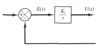
Integral control action. In a controller with integral control action, the value of the controller output is changed at a rate proportional to the actuating error signal That is,

Figure 5-6 Block diagram of a proportional controller.

or

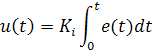
where is an adjustable constant.The transfer function of the integral controller is

If the value of is doubled, then the value of varies twice as fast. For zero actuating error, the value of remains stationary. The integral control action is sometimes called reset control. Figure 5-7 shows a block diagram of such a controller.

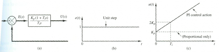
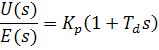
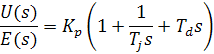
Proportional-plus-integral control action. The control action of a proportional-plus-integral controller is defined by

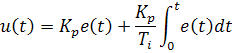
or the transfer function of the controller is

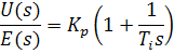
where is the proportional gain, and T, is called the integral time. Both and are adjustable. The integral time adjusts the integral control action, while a change in the value of affects both the proportional and integral parts of the control action. The inverse of the integral time is called the reset rate. The reset rate is the number of times per minute that the proportional part of the control action is duplicated. Reset rate is measured in terms of repeats per minute. Figure 5-8 (a) shows a block diagram of a proportional-plus-integral controller. If the actuating error signal is a unit-step function as shown in Figure 5-8(b), then the controller output becomes as shown 1 in Figure 5-8(c).

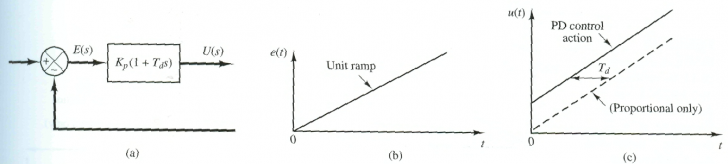
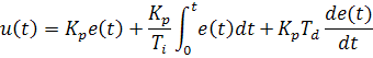
Proportional-plus-derivative control action. The control action of a proportional plus-derivative controller is defined by

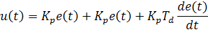
and the transfer function is

Figure 5-7 Block diagram of an integral controller

Figure 5-8 a) Block diagram of a proportional-plus-integral controller; (b) and

(c) diagrams depicting a unit-step input and the controller output.

where is the proportional gain and is a constant called the derivative time. Both and are adjustable. The derivative control action, sometimes called rate control, is where the magnitude of the controller output is proportional to the rate of change of the actuating error signal. The derivative time is the time interval by which the rate action advances the effect of the proportional control action. Figure 5-9(a) shows a block diagram of a proportional-plus-derivative controller. If the actuating error signal is a unit-ramp function as shown in Figure 5-9(b), then the controller output becomes as shown in Figure 5-9(c). As may be seen from Figure 5-9(c), the derivative control action has an anticipatory character. As a matter of course, however, derivative control action can never anticipate any action that has not yet taken place.

While derivative control action has the advantage of being anticipatory, it has the disadvantages that it amplifies noise signals and may cause a saturation effect in the actuator.

Note that derivative control action can never be used alone because this control action is effective only during transient periods.

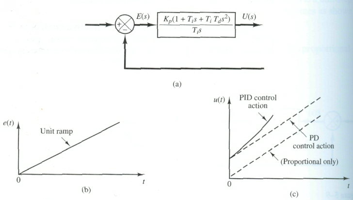
Proportional-plus-integral-plus-derivative control action. The combination of proportional control action, integral control action, and derivative control action is termed proportional-plus-integral-plus-derivative control action. This combined action

Figure 5-9 (a) Block diagram of a proportional-plus-derivative controller; (b) and (c) diagrams depicting a unit-ramp input and the controller output.

has the advantages of each of the three individual control actions. The equation of a controller with this combined action is given by

or the transfer function is

where is the proportional gain, is the integral time, and is the derivative time. The block diagram of a proportional-plus-integral-plus-derivative controller is shown j in Figure 5-10(a). If is a unit-ramp function as shown in Figure 5-10(b), then the] controller output becomes as shown in Figure 5-10(c).

Effects of the sensor (measuring element) on system performance. Since

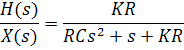
the dynamic and static characteristics of the sensor or measuring element affect the indication of the actual value of the output variable, the sensor plays an important role in determining the overall performance of the control system. The sensor usually determines the transfer function in the feedback path. If the time constants of a sensor are negligibly small compared with other time constants of the control system, the transfer function of the sensor simply becomes a constant. Figures 5-11(a), (b), and (c) show block diagrams of automatic controllers having a first-order sensor, an overdamped second-order sensor, and an underdamped second-order sensor* respectively. The response of a thermal sensor is often of the overdamped second order type.

Figure 5-10 (a) Block diagram of a proportional-plus-integral-plus-derivative controller; (b) and (c) diagrams depicting a unit-ramp input and the controller output.

3. EFFECTS OF INTEGRAL AND DERIVATIVE CONTROL ACTIONS ON SYSTEM PERFORMANCE

In this section, we shall investigate the effects of integral and derivative control actions on the system performance. Here we shall consider only simple systems so that the effects of integral and derivative control actions on system performance can be clearly seen.

Integral control action. In the proportional control of a plant whose transfer function does not possess an integrator 1/s, there is a steady-state error, or offset, in the response to a step input. Such an offset can be eliminated if the integral control action is included in the controller.

In the integral control of a plant, the control signal, the output signal from the controller, at any instant is the area under the actuating error signal curve up to that instant. The control signal can have a nonzero value when the actuating error signal is zero, as shown in Figure 5-12(a).This is impossible in the case of the proportional controller since a nonzero control signal requires a nonzero actuating error signal. (A nonzero actuating error signal at steady state means that there is an offset.) Figure 5-12(b) shows the curve versus t and the corresponding curve versus when the controller is of the proportional type.

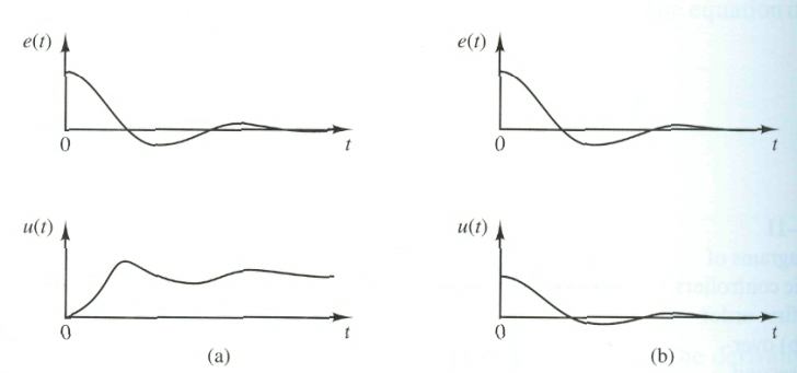
Note that integral control action, while removing offset or steady-state error, may lead to oscillatory response of slowly decreasing amplitude or even increasing amplitude, both of which are usually undesirable.

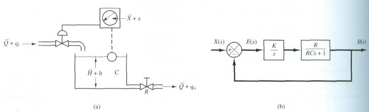
Integral control of liquid-level control systems. In Section 4-2, we found that the proportional control of a liquid-level system will result in a steady-state error with a step input. We shall now show that such an error can be eliminated if integral control action is included in the controller.

Figure 5-12 (a) Plots of and curves showing nonzero control signal when the actuating error signal is zero (integral control); (b) plots of and curves showing zero control signal when the actuating error signal is zero (proportional control).

Figure 5-13(a) shows a liquid-level control system. We assume that the controller is an integral controller. We also assume that the variables h, and which are measured from their respective steady-state values and are small quantities so that the system can be considered linear. Under these assumptions, the block diagram of the system can be obtained as shown in Figure 5-13(b). From Figure 5-13(b), the closed-1 loop transfer function between and is

Hence

Since the system is stable, the steady-state error for the unit-step response is obtained by applying the final-value theorem, as follows:

Figure 5-13 (a) Liquid-level control system; (b) block diagram of the system.

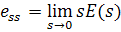
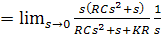
Integral control of the liquid-level system thus eliminates the steady-state error in the response to the step input. This is an important improvement over the proportional control alone, which gives offset.

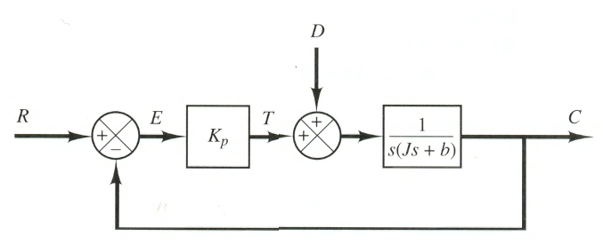
Response to torque disturbances (proportional control). Let us investigate the effect of a torque disturbance occurring at the load element. Consider the system shown in Figure 5-14. The proportional controller delivers torque to position the load element, which consists of moment of inertia and viscous friction. Torque disturbance is denoted by

Assuming that the reference input is zero or , the transfer function between and is given by

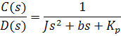
Hence

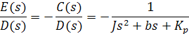
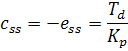
The steady-state error due to a step disturbance torque of magnitude is given by

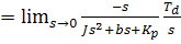
At steady state, the proportional controller provides the torque - which is equal in magnitude but opposite in sign to the disturbance torque The steady-state output due to the step disturbance torque is

Figure 5-14 Control system with a torque disturbance.