| CATEGORII DOCUMENTE |
| Bulgara | Ceha slovaca | Croata | Engleza | Estona | Finlandeza | Franceza |
| Germana | Italiana | Letona | Lituaniana | Maghiara | Olandeza | Poloneza |
| Sarba | Slovena | Spaniola | Suedeza | Turca | Ucraineana |
 EN222:
Mechanics of Solids
EN222:
Mechanics of SolidsDivision of Engineering
Fracture Mechanics
The goal of fracture mechanics is to predict the critical loads that will cause catastrophic failure in a structure or component. It is a large and venerable field with many sub-disciplines. Some of these are illustrated schematically in the picture below
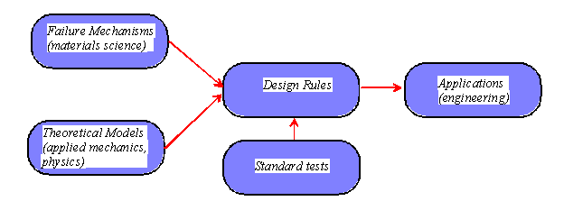
The ultimate goal of work in the field is to be able to design structures or components that are capable of withstanding cyclic or static service loads. Most engineering decisions are based on semi-empirical design rules, which rely on phenomenological fracture or fatigue criteria calibrated by means of standard tests. The design rules are based on current understanding of how materials fail, which is derived from extensive observations of failure mechanisms, together with theoretical models that have been developed to describe, as far as possible, these mechanisms of failure.
The mechanisms involved in fracture or fatigue failure are complex, and is influenced by material and structural features that span 12 orders of magnitude in length scale.
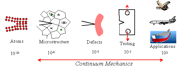
Continuum mechanics contributes to understanding of failure mechanisms from the sub-micron to km length scales. Most engineering applications involve structures of the order of mm-km. For many such applications, its sufficient to measure the maximum cyclic or static stress (or perhaps strain) that the material can withstand, and then design the structure to ensure that the stress (or strain) remains below acceptable limits. This involves fairly routine constitutive modeling and numerical or analytical solution of appropriate boundary value problems. More critical applications require some kind of defect tolerance analysis perhaps the material or structure is known to contain flaws, and the engineer must decide whether to replace the part; or perhaps it is necessary to specify material quality standards. This kind of decision is usually made using either linear elastic, or plastic, fracture mechanics. Finally, there is great interest in designing failure resistant materials. In this case the basic question is: how does the material fail, and what can be done to the materials microstructure to avoid failure? This is a more exploratory field, but continuum mechanics has provided insight into a range of issues in this area.
We do not have time to address all these issues in this course. Instead, we will summarize some results in the continuum mechanics of solids that are central to analysis of fracture and fatigue, and outline briefly their main applications. Specifically, we will give
In order to understand the various approaches to modeling fracture, fatigue and failure, it is helpful to review briefly the features and mechanisms of failure in solids.
If you test a sample of any material under uniaxial tension it will eventually fail. The features of the failure depend on several factors, including
![]() The materials involved and their microsctructure;
The materials involved and their microsctructure;
![]() The applied stress state (particularly the hydrostatic stress)
The applied stress state (particularly the hydrostatic stress)
![]() Loading rate
Loading rate
![]() Temperature
Temperature
![]() Ambient environment (water vapor; or presence of
corrosive environments.
Ambient environment (water vapor; or presence of
corrosive environments.
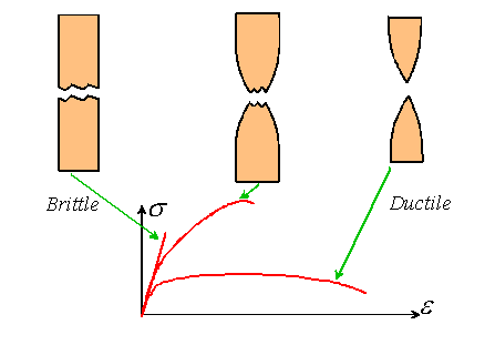
Materials are normally classified loosely as either `brittle or `ductile depending on the characteristic features of the failure. Examples of `brittle materials include refractory oxides (ceramics) and intermetallics, as well as BCC metals at low temperature (below about of the melting point). Features of a brittle material are
Examples of `ductile materials include FCC metals at all temperatures; BCC metals at high temperatures; polymers at high temperature. Features of a `ductile fracture are
Of course, some materials have such a complex microstructure (especially composites) that its hard to classify them as entirely brittle or entirely ductile.
Brittle fracture occurs as a result of a single crack propagating through the specimen. Some materials contain pre-existing cracks, in which case fracture is initiated when a large crack in a region of high tensile stress starts to grow. In other materials, the origin of the fracture is less clear various mechanisms for nucleating crack have been suggested, including dislocation pile-up at grain boundaries; or intersections of dislocations.
Ductile fracture occurs as a result of the nucleation, growth and coalescence of voids in the material. Failure is controlled by the rate of nucleation of the voids; their rate of growth, and the mechanism of coalescence. High tensile hydrostatic stress promotes rapid void nucleation and growth, but void growth generally also requires significant bulk plastic strain.
A ductile material may also fail as a result of plastic instability such as necking, or the formation of a shear band. This is analogous to buckling at a critical strain, the component no longer deforms uniformly, and the deformation localizes to a small region of the solid. This is normally accompanied by a loss of load bearing capacity and a large increase in plastic strain rate in the localized region, which normally results in failure.
Some materials, especially brittle materials such as glasses, and oxide based ceramics, suffer from a form of time-delayed failure under steady loading, known as `static fatigue. Automatic coffee-maker jugs are particularly susceptible to static fatigue. You use one for a couple of years, and then one day it shatters if you tap it against the side of the sink. This is because the jugs strength has degraded with time. Static fatigue in brittle materials is a consequence of corrosion crack growth. The highly stressed material near a crack tip is particularly susceptible to chemical attack (the stress increases the rate of chemical reaction). Material near the crack tip may be dissolved altogether, or it may form a reaction product with very low strength. In either event, the crack slowly propagates through the solid, until it becomes long enough to trigger brittle fracture. Glasses and oxide based ceramics are particularly susceptible to attack by water-vapor (and perhaps coffee).
Mechanical engineers generally have to design components to withstand cyclic as opposed to static loading. Fatigue failure is a familiar phenomenon, but a detailed understanding of the mechanisms involved and the ability to model them quantitatively have only emerged in the past 50 years, driven largely by the demands of the aerospace industry. There are some forms of fatigue failure (contact fatigue is an example) where the mechanisms involved are still a mystery.

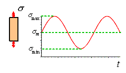
Fatigue life is measured by subjecting the material to cyclic loading. Usually the loading is uniaxial tension, although other cycles are used too (e.g. contact fatigue applications). The cycle can be stress controlled, or strain controlled. A cycle of uniaxial load is characterized by
![]() The stress amplitude
The stress amplitude ![]()
![]()
![]()
![]()
![]()
![]() The mean stress
The mean stress ![]()

![]()
![]()
![]()
![]() The stress ratio
The stress ratio ![]()
![]()
![]()
![]()
![]()
A
rotating bending test is a particularly convenient way to subject a material to
a very large number of cycles in a short period of time. The shaft can
easily be spun at 2000rpm, allowing the material to be subjected to ![]()
![]()
![]()
![]()
![]() cycles
in less than 100 hrs. Pulsating tension is more common in service
loading, but a servo-hydraulic tensile testing machine operating at 1Hz takes
nearly 4 months to complete
cycles
in less than 100 hrs. Pulsating tension is more common in service
loading, but a servo-hydraulic tensile testing machine operating at 1Hz takes
nearly 4 months to complete ![]()
![]()
![]()
![]()
![]() cycles.
cycles.

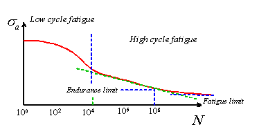
The
resistance of a material to cyclic loading is characterized by plotting an
`S-N curve showing the number of cycles to failure as a function of stress.
The plot normally shows different regimes of behavior, depending on stress
amplitude. At high stress levels, the material deforms plastically and
fails rapidly. In this regime the life of the specimen depends primarily
on the plastic strain amplitude, rather than the stress amplitude. This
is referred to as `low cycle fatigue behavior. At lower stress levels
life has a power law dependence on stress this is referred to as `high cycle
fatigue behavior. In some materials, there is a clear fatigue limit
if the stress amplitude lies below a certain limit, the specimen remains
intact forever. In other materials there is no clear fatigue
threshold. In this case, the stress amplitude at which the material
survives ![]()
![]()
![]()
![]()
![]() cycles
is taken as the endurance limit of the material.
cycles
is taken as the endurance limit of the material.
Fatigue life is sensitive to the mean stress, or R ratio, and tends to fall rather rapidly as R increases. It is also influenced by environment, and temperature, and can be very sensitive to details such as the surface finish of the specimen.
A
tensile specimen that has failed by fatigue looks at first sight as though it
has failed by brittle fracture. The fracture surface is flat, and the two
sides of the specimen fit together quite well. In fact, for some time it
was thought that some bizarre metallurgical process was responsible for turning
a ductile material brittle under cyclic loading. (An engineer named Nevil
Fatigue failures are caused by slow crack growth through the material. The failure process involves four stages
1. Crack initiation
2. Micro-crack growth (with crack length less than the materials grain size) (Stage I)
3. Macro crack growth (crack length between 0.1mm and 10mm) (Stage II)
4. Failure by fast fracture.
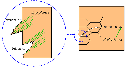
Cracks will generally only initiate in the presence of cyclic plasticity. However, bulk plastic flow in the specimen is not necessary: plastic flow may be caused by local stress concentrations at notches in the part, due to geometric defects such as dents or scratches in the surface or even due to microstructural features such as large inclusions in the material. In a smooth, clean specimen, the cracks form where `persistent slip bands reach the surface of the specimen. Plastic flow in a material is generally highly inhomogeneous at the micron scale, with the deformation confined to narrow localized bands of slip. Where these bands intersect the surface, intrusions or extrusions form, which serve as nucleation sites for cracks.
Cracks initially propagate along the slip bands at around 45 degrees to the principal stress direction this is known as Stage I fatigue crack growth. When the cracks reach a length comparable to the materials grain size, they change direction and propagate perpendicular to the principal stress. This is known as Stage II fatigue crack growth.
The simplest brittle fracture criterion states that fracture is initiated when the greatest tensile principal stress in the solid reaches a critical magnitude,
![]()
![]()
![]()
![]()
![]()
(The subscript TS stands for tensile strength).
To
apply the criterion, you must first measure (or look up) ![]()
![]()
![]()
![]()
![]() for
the material.
for
the material. ![]()
![]()
![]()
![]()
![]() can be measured by conducting tensile tests on specimens
it is important to test a large number of specimens because the failure stress
is likely to show a great deal of statistical scatter. The tensile
strength can also be measured using beam bending tests. The failure
stress measured in a bending test is referred to as the `modulus of rupture
can be measured by conducting tensile tests on specimens
it is important to test a large number of specimens because the failure stress
is likely to show a great deal of statistical scatter. The tensile
strength can also be measured using beam bending tests. The failure
stress measured in a bending test is referred to as the `modulus of rupture ![]()
![]()
![]()
![]()
![]() for
the material. It is nominally equivalent to
for
the material. It is nominally equivalent to ![]()
![]()
![]()
![]()
![]() but
in practice usually turns out to be somewhat higher.
but
in practice usually turns out to be somewhat higher.
Then
you must calculate the anticipated stress distribution in your component or
structure (e.g. using FEM). Finally, you plot contours of principal
stress, and find the maximum value ![]()
![]()
![]()
![]()
![]() .
If
.
If ![]()
![]()
![]()
![]()
![]() the
design is safe (but be sure to use an appropriate factor of safety!).
the
design is safe (but be sure to use an appropriate factor of safety!).
Probabilistic Design Methods for Brittle Fracture Weibull Statistics)
The
fracture criterion ![]()
![]()
![]()
![]()
![]() is
too crude for many applications. The tensile strength of a brittle solid
usually shows considerable statistical scatter, because the likelihood of
failure is determined by the probability of finding a large flaw in a highly
stressed region of the material. This makes it difficult to determine an
unambiguous value for tensile strength should you use the median value of
your experimental data? (no way!). Pick the
stress level where 95% of specimens survive? (Better!). Its better
to deal with this problem using a more rigorous statistical approach.
is
too crude for many applications. The tensile strength of a brittle solid
usually shows considerable statistical scatter, because the likelihood of
failure is determined by the probability of finding a large flaw in a highly
stressed region of the material. This makes it difficult to determine an
unambiguous value for tensile strength should you use the median value of
your experimental data? (no way!). Pick the
stress level where 95% of specimens survive? (Better!). Its better
to deal with this problem using a more rigorous statistical approach.

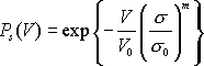
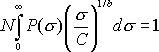
Weibull
statistics refers to a technique used to predict the probability of failure of
a brittle material. The approach is to test a large number of samples
with identical size and shape under uniform tensile stress, and determine the
survival probability as a function of stress (survival probability is
approximated by the fraction of specimens that survive a given stress
level). The survival probability ![]()
![]()
![]()
![]()
![]() is
fit by a Weibull distribution
is
fit by a Weibull distribution

![]()
![]()
![]()
![]()
where
![]()
![]()
![]()
![]()
![]() is
the volume of the specimen, and
is
the volume of the specimen, and ![]()
![]()
![]()
![]()
![]() , m
are material constants. The index m is typically of the order 5-10
for ceramics, and is independent of specimen volume. The parameter
, m
are material constants. The index m is typically of the order 5-10
for ceramics, and is independent of specimen volume. The parameter ![]()
![]()
![]()
![]()
![]() is
the stress at which the probability of survival is exp(-1), (about 37%). This
does vary with specimen volume.
is
the stress at which the probability of survival is exp(-1), (about 37%). This
does vary with specimen volume.
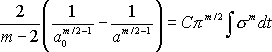
Given
m, ![]()
![]()
![]()
![]()
![]() and
the corresponding specimen volume
and
the corresponding specimen volume ![]()
![]()
![]()
![]()
![]() ,
the survival probability of a volume
,
the survival probability of a volume ![]()
![]()
![]()
![]()
![]() of
material subjected to uniform uniaxial stress
of
material subjected to uniform uniaxial stress ![]()
![]()
![]()
![]()
![]() follows
as
follows
as
![]()
![]()
![]()
![]()
To
see this, note that the volume V can be thought of as containing ![]()
![]()
![]()
![]()
![]() specimens.
The probability that they all survive is
specimens.
The probability that they all survive is ![]()
![]()
![]()
![]()
![]() .
.
The
survival probability of a solid subjected to an arbitrary stress distribution
with principal values ![]()
![]()
![]()
![]()
![]() can
be computed as
can
be computed as
![]()
![]()
![]()
![]()
![]()
where
![]()
![]()
![]()
![]()
![]()
This approach is quite successful in some applications, for example, it explains why brittle materials appear to be stronger in bending than in uniaxial tension. Like many statistical approaches it has some limitations as a design tool. The problem is that we can predict quite nicely the stress that gives 30% probability of failure. But who the hell buys a product that has a 30% probability of failure? (Yeah, I know Microsoft users). For design applications we need to predict the probability of 1 failure in a million or so. It is very difficult to measure the tail of a statistical distribution accurately, and a distribution that was fit to predict 63% failure probability may be wildly inaccurate in the region of interest.
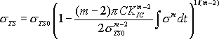
A
fracture mechanics approach (discussed in more detail below, where we address
the mechanics of cracks) can be used to develop a suitable phenomenological
static fatigue law. We assume that at time t=0 the material
contains a crack of initial length 2 ![]()
![]()
![]()
![]()
![]() ,
and is subjected to a stress
,
and is subjected to a stress ![]()
![]()
![]()
![]()
![]() .
The stress will cause the crack to increase in length, until it becomes long
enough to trigger brittle fracture. A corrosion crack grows at a rate
determined by the crack tip stress intensity factor
.
The stress will cause the crack to increase in length, until it becomes long
enough to trigger brittle fracture. A corrosion crack grows at a rate
determined by the crack tip stress intensity factor ![]()
![]()
![]()
![]()
![]() -
well define this shortly, but for present purposes it is sufficient to know that
for a crack of length 2a subjected to stress
-
well define this shortly, but for present purposes it is sufficient to know that
for a crack of length 2a subjected to stress ![]()
![]()
![]()
![]()
![]() the
stress intensity factor is
the
stress intensity factor is ![]()
![]()
![]()
![]()
![]() .
Experiments suggest that the crack growth rate can be approximated by
.
Experiments suggest that the crack growth rate can be approximated by
![]()
![]()
![]()
![]()
![]()
where m is of order 10-20. We therefore obtain the following expression for crack length as a function of time
![]()
![]()
![]()
![]()
where
2 ![]()
![]()
![]()
![]()
![]() is
the crack length at time t=0. The solid will fracture when
the crack tip stress intensity factor reaches a critical value
is
the crack length at time t=0. The solid will fracture when
the crack tip stress intensity factor reaches a critical value ![]()
![]()
![]()
![]()
![]() , so
that the tensile strength at time t=0 and at time t
satisfy
, so
that the tensile strength at time t=0 and at time t
satisfy
![]()
![]()
![]()
![]()
![]()
Eliminating the crack length and simplifying gives
![]()
![]()
![]()
![]()
Assuming that the operating stress is well below the fracture stress, we can approximate this by
![]()
![]()
![]()
![]()
![]()
where ![]()
![]()
![]()
![]()
![]() is
a constitutive parameter, to be determined by experiment. For a component that
is subjected to a constant operating stress
is
a constitutive parameter, to be determined by experiment. For a component that
is subjected to a constant operating stress
![]()
![]()
![]()
![]()
![]()
This
expression can be used in design calculations to estimate the degradation in
tensile strength (or the Weibull stress ![]()
![]()
![]()
![]()
![]() , if
you prefer) with time. The constants
, if
you prefer) with time. The constants ![]()
![]()
![]()
![]()
![]() and
m must be determined from experiment.
and
m must be determined from experiment.
Note
that the structure fails when ![]()
![]()
![]()
![]()
![]() ,
giving
,
giving
![]()
![]()
![]()
![]()
for the time to failure. Thus, m and ![]()
![]()
![]()
![]()
![]() can
be conveniently determined by measuring the time to failure of a material as a
function of stress under constant loading.
can
be conveniently determined by measuring the time to failure of a material as a
function of stress under constant loading.
Brittle materials are generally used in applications where they are subjected primarily to compressive stress. Brittle materials are very strong in compression, but they will fail if subjected to combined hydrostatic compression and shear (e.g. by loading in uniaxial compression). Failure in compression is a consequence of distributed microcracking in the solid large numbers of small cracks form, propagate for a short while and then arrest. Failure occurs as a result of coalescence of these cracks. Failure in compression is less catastrophic than tension, and in some respects qualitatively resembles metal plasticity.
This type of crushing is usually modeled using an extended classical plasticity theory. Its most common application is to model concrete. A simple constitutive law of this type has the form
1. Decomposition of strain into elastic and irreversible (damage) parts ![]()
![]()
![]()
![]()
![]()
2. A pressure dependent failure surface of the form
![]()
![]()
![]()
![]()
![]()
where
![]()
![]()
![]()
![]()
![]() ,
, ![]()
![]()
![]()
![]()
![]() , c
is a material constant controlling the variation of strength with hydrostatic
pressure,
, c
is a material constant controlling the variation of strength with hydrostatic
pressure, ![]()
![]()
![]()
![]()
![]() is
the accumulated irreversible strain, and
is
the accumulated irreversible strain, and ![]()
![]()
![]()
![]()
![]() is
a functional fit to the stress strain curve in uniaxial compression;
is
a functional fit to the stress strain curve in uniaxial compression;
3. An associated flow rule
![]()
![]()
![]()
![]()
![]()
These
constitutive equations are used only in regions where the hydrostatic stress is
compressive ![]()
![]()
![]()
![]()
![]() .
.
In regions of hydrostatic tension, a tensile brittle fracture criterion should be used for example, the material could be assumed to lose all load bearing capacity if the principal tensile stress exceeds a critical magnitude.
Ductile fracture in tension occurs by the nucleation, growth and coalescence of voids in the material. A crude criterion for ductile failure could be based on the accumulated plastic strain, for example
![]()
![]()
![]()
![]()
![]()
at failure, where ![]()
![]()
![]()
![]()
![]() is
the plastic strain to failure in a uniaxial tensile test.
is
the plastic strain to failure in a uniaxial tensile test.
This failure criterion does not account for the substantial reduction in strength caused by the presence of tensile hydrostatic stress. A more sophisticated approach uses a state variable plasticity law, in which the void volume fraction is an explicit state variable.
![]()
![]()
![]()
![]()
where
![]()
![]()
![]()
![]()
![]() is
a functional fit to the uniaxial stress-strain curve of the fully dense
material (
is
a functional fit to the uniaxial stress-strain curve of the fully dense
material ( ![]()
![]()
![]()
![]()
![]() ),
),
![]()
![]()
![]()
![]()
![]() and
and
![]()
![]()
![]()
![]()
![]() .
More recent variants introduce a few more adjustable parameters in the yield
function to provide a better fit to numerical simulations of voided materials.
Note that the yield stress is pressure dependent (decreasing with hydrostatic
tension), and the yield stress decreases as the volume fraction of voids
increases, dropping to zero at
.
More recent variants introduce a few more adjustable parameters in the yield
function to provide a better fit to numerical simulations of voided materials.
Note that the yield stress is pressure dependent (decreasing with hydrostatic
tension), and the yield stress decreases as the volume fraction of voids
increases, dropping to zero at ![]()
![]()
![]()
![]()
![]() .
The uniaxial stress strain curve
.
The uniaxial stress strain curve ![]()
![]()
![]()
![]()
![]() for
a porous plastic metal would have to be determined from a compression
test on the fully dense solid, because in a tension test youd nucleate voids
and consequently underestimate the yield stress.
for
a porous plastic metal would have to be determined from a compression
test on the fully dense solid, because in a tension test youd nucleate voids
and consequently underestimate the yield stress.
The model uses an associated flow law
![]()
![]()
![]()
![]()
![]()
where ![]()
![]()
![]()
![]()
![]() is
the magnitude of the plastic strain increment and
is
the magnitude of the plastic strain increment and ![]()
![]()
![]()
![]()
![]() is
a constant, which must be determined from a consistency condition on the
plastic dissipation
is
a constant, which must be determined from a consistency condition on the
plastic dissipation
![]()

![]()
which yields a scalar equation that can be solved for C.
Finally, the model is completed by specifying the void volume fraction as a function of strain. The void volume fraction can increase due to nucleation of new voids, or due to growth of existing voids. The void volume fraction can also decrease if the voids are closed up by compressive straining. To account for both effects, one can set
![]()
![]()
![]()
![]()
![]()
where the first term accounts for void growth, and the second accounts for strain controlled void nucleation. Any sensible function can be used for A (its very difficult to determine experimentally). You could assume the voids nucleate at a uniform rate. A more sophisticated approach might be to assume that the void nucleation rate initially increases with plastic strain, reaches a maximum at some critical strain, and then drops off again as the void nucleation sites are exhausted.
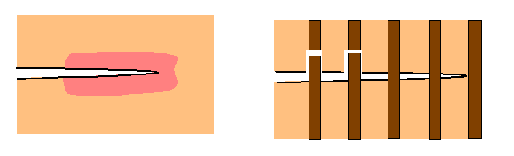
If you test a cylindrical specimen of a very ductile material in uniaxial tension, it will initially deform uniformly. At a critical load the specimen will start to neck, as shown in the picture. Necking, once it starts, is usually unstable there is a concentration in stress near the necked region, increasing the rate of plastic flow near the neck compared with the rest of the specimen, and so increasing the rate of neck formation. The strains in the necked region rapidly become very large, which will quickly lead to failure.
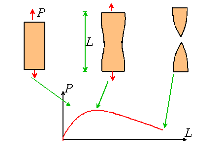
Neck formation is a consequence of geometric softening. A very simple model explains the concept of geometric softening. Consider a cylindrical specimen with cross sectional area A. Assume that the material is perfectly plastic and has a true stress-strain curve (Cauchy stress v- logarithmic strain) that can be approximated by a power-law
![]()
![]()
![]()
![]()
![]()
with n<1. Suppose
that at some time t the specimen is subjected to a load P, and
has length L, strain ![]()
![]()
![]()
![]()
![]() and
cross sectional area A. We now increase the length of the
specimen by an infinitesimal displacement dL. This causes an
increment in Logarithmic strain
and
cross sectional area A. We now increase the length of the
specimen by an infinitesimal displacement dL. This causes an
increment in Logarithmic strain ![]()
![]()
![]()
![]()
![]() ,
increasing the Cauchy stress to
,
increasing the Cauchy stress to ![]()
![]()
![]()
![]()
![]() .
At the same time, the cross sectional area of the bar decreases to
.
At the same time, the cross sectional area of the bar decreases to ![]()
![]()
![]()
![]()
![]() .
(To see this note that
.
(To see this note that
![]()
![]()
![]()
![]()
![]()
The first term is the result of strain hardening, and tends to increase the load. The second term is a consequence of the lateral contraction of the bar, and tends to decrease the load. This second term is referred to as geometric softening the effect of the specimens geometry is to reduce the load required to stretch the specimen.
Notice that there is a critical critical strain ![]()
![]()
![]()
![]()
![]() such
that
such
that
![]()
![]()
![]()
![]()
![]()
Consequently, the load reaches a peak value at strain ![]()
![]()
![]()
![]()
![]() ,
and the maximum load the specimen can withstand follows as
,
and the maximum load the specimen can withstand follows as
![]()
![]()
![]()
![]()
![]()
where ![]()
![]()
![]()
![]()
![]() is
the initial cross sectional area of the bar.
is
the initial cross sectional area of the bar.
It turns out that the point of maximum load coincides with the condition for unstable neck formation in the bar. This is plausible a falling load displacement curve is always a sign that there might be a possibility of non-unique solutions but a rather sophisticated calculation is required to show this rigorously.
There are two important points to take away from this discussion.
![]() Plastic localization, as opposed to material failure, may limit load bearing
capacity
Plastic localization, as opposed to material failure, may limit load bearing
capacity
![]() If you measure the strain to failure of a material in uniaxial tension, it is
possible that you have learned absolutely nothing about the inherent strength
of the material your specimen may have failed due to a geometric effect;
If you measure the strain to failure of a material in uniaxial tension, it is
possible that you have learned absolutely nothing about the inherent strength
of the material your specimen may have failed due to a geometric effect;
Plastic localization can occur for many reasons. There are two general classes of localization it may occur as a consequence of changes in specimen geometry (i.e. geometric softening); or it may occur due to a natural tendency of the material itself to soften at large strains.
Examples of geometry induced localization are
(i) Neck formation in a bar under uniaxial tension;
(ii) Shear band formation in torsional or shear loading at high strain rate due to thermal softening as a result of plastic heat generation
Examples of material induced localization are
(i) Localization in a Gurson solid due to the softening effect of voids at large strains;
(ii) Localization in a single crystal due to the softening effect of lattice rotations;
(iii) Localization in a brittle microcracking material due to the reduction in elastic compliance caused by the cracks.
From a modeling standpoint, localization is the easiest form of failure to deal with, because it does not rely on any empirical failure criteria. A straightforward FEM computation, with an appropriate constitutive law and proper consideration of finite strains, will predict localization if it is going to occur the only thing you need to worry about is to be sure you understand what triggered the localization. Localization can start at a geometric imperfection in the model, in which case your prediction is meaningful (but may be sensitive to the nature of the imperfection). It may also be triggered by numerical errors, in which case the predicted failure load is meaningless. It is usually exceedingly difficult to compute what happens after localization. Fortunately its rather rare to need to do this for design purposes.
High Cycle Fatigue
Empirical stress or strain based life prediction methods are extensively used in design applications. The approach is straightforward subject a sample of the material to a cycle of stress (or strain) that resembles service loading, in an environment representative of service conditions, and measure its life as a function of stress (or strain) amplitude.
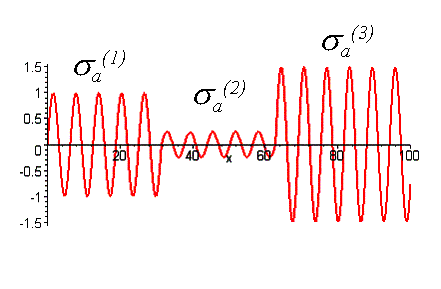
Here
we will review criteria that are used to predict fatigue life under
proportional cyclic loading. A typical stress cycle is parameterized by its
amplitude ![]()
![]()
![]()
![]()
![]() and
the mean stress
and
the mean stress ![]()
![]()
![]()
![]()
For
tests run in the high cycle fatigue regime with any fixed value of mean stress,
the relationship between stress amplitude ![]()
![]()
![]()
![]()
![]() and
the number of cycles to failure N is fit well by Basquins Law
and
the number of cycles to failure N is fit well by Basquins Law
![]()
![]()
![]()
![]()
![]()
where the exponent b is typically between 0.05 and 0.15. The constant C is a function of mean stress.
There are two ways to account for the effects of mean stress. Both are based on the same idea: we know that if the mean stress is equal to the tensile strength of the material, it will fail in 0 cycles of loading. We also know that for zero mean stress, the fatigue life obeys Basquins law. We can interpolate between these two points.
Goodmans rule uses a linear interpolation, giving
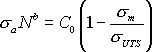
![]()
![]()
![]()
![]()
where
![]()
![]()
![]()
![]()
![]() is
the constant in Basquins law determined by testing at zero mean stress.
is
the constant in Basquins law determined by testing at zero mean stress.
Gerbers rule uses a parabolic fit
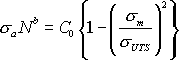
![]()
![]()
![]()
![]()
In practice, experimental data seem to lie between these two limits. Goodmans rule gives a safe estimate.
Low Cycle Fatigue
If a fatigue test is run with a high stress level (sufficient to cause plastic flow) the specimen fails very quickly (less than 10 000 cycles). This regime of behavior is known as `low cycle fatigue. The fatigue life correlates best with the plastic strain amplitude rather than stress amplitude, and it is found that the Coffin Manson Law
![]()
![]()
![]()
![]()
![]()
gives a good fit to empirical data (the constant C and b do not have the same values as for Basquins law, of course)
Fatigue tests are usually done at constant stress (or strain) amplitude. Service loading usually involves cycles with variable (and often random) amplitude. Fortunately, theres a remarkably simple way to estimate fatigue life under variable loading using constant stress data.
Suppose
the load history is comprised of a set of ![]()
![]()
![]()
![]()
![]() load
cycles at a stress amplitude
load
cycles at a stress amplitude ![]()
![]()
![]()
![]()
![]() ,
followed by a set of
,
followed by a set of ![]()
![]()
![]()
![]()
![]() cycles
at load amplitude
cycles
at load amplitude ![]()
![]()
![]()
![]()
![]() and
so on. For the ith set of cycles at load amplitude
and
so on. For the ith set of cycles at load amplitude ![]()
![]()
![]()
![]()
![]() , we
could compute the number of cycles that would cause the specimen to fail using
Basquins law
, we
could compute the number of cycles that would cause the specimen to fail using
Basquins law
![]()
![]()
![]()
![]()
![]()
The Miner-Palmgren failure criterion assumes a linear summation of damage due to each set of load cycles, so that
![]()
![]()
![]()
![]()
![]()
at failure. In terms of stress amplitude
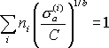
![]()
![]()
![]()
![]()
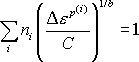
![]()
![]()
![]()
![]()
![]()
![]()
![]()
![]()
Phenomenological damage models are useful in design applications, but they have many limitations, including
![]() They
require extensive experimental testing to calibrate the model for each
application;
They
require extensive experimental testing to calibrate the model for each
application;
![]() They
provide no insight into the relationship between a materials microstructure and
its strength;
They
provide no insight into the relationship between a materials microstructure and
its strength;
A more sophisticated approach is to model the mechanisms of failure directly. Crack propagation through the solid, either as a result of fatigue, or by brittle or ductile fracture, is by far the most common cause of failure. Consequently much effort has been devoted to developing techniques to predict the behavior of cracks in solids. Below, we outline some of the most important results.
Crack Tip Fields in homogeneous Elastic Solids.
Many of the techniques of fracture mechanics rely on the assumption that, if one gets sufficiently close to the tip of the crack, the stress, displacement and strain fields always look the same (differing only in magnitude). The fields near a crack tip are a fundamental result in fracture mechanics.
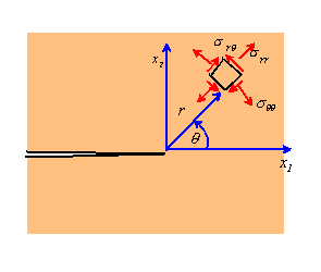
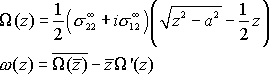
The state of stress can be calculated by considering a semi-infinite crack in an infinite elastic solid subjected to uniform loading at infinity.
For anti-plane shear loading, the displacement can be computed from a complex potential (following the procedure outlined in Section 4) as
![]()
![]()
![]()
![]()
![]()
where
C is a constant and ![]()
![]()
![]()
![]()
![]() .
The stress state follows as
.
The stress state follows as
![]()
![]()
![]()
![]()
![]()
Evidently this solution satisfies all boundary conditions for all values of C. As expected, the stress distribution is known, but its magnitude is arbitrary. It is conventional to re-scale the stress and displacement fields by defining the mode III stress intensity factor
![]()
![]()
![]()
![]()
![]()
giving
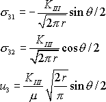

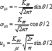

![]()
for the stress and displacement fields.
The equivalent plane problem is most conveniently derived from an Airy function. The derivation is outlined in detail in the linear elasticity notes. It is found that the Airy function
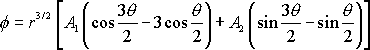
![]()
![]()
![]()
![]()
(with
![]()
![]()
![]()
![]()
![]() arbitrary
constants) generates a solution satisfying traction free boundary conditions on
the crack faces; with vanishing stress at infinity and bounded strain
energy. The stress state is singular at the crack tip, just like
the equivalent anti-plane shear solution. The unknown stress
magnitude is scaled by introducing Mode I and Mode II stress intensity factors
arbitrary
constants) generates a solution satisfying traction free boundary conditions on
the crack faces; with vanishing stress at infinity and bounded strain
energy. The stress state is singular at the crack tip, just like
the equivalent anti-plane shear solution. The unknown stress
magnitude is scaled by introducing Mode I and Mode II stress intensity factors
![]()
![]()
![]()
![]()
![]()
The stresses follow from the Airy function as
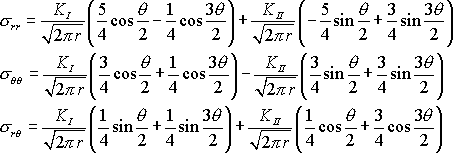


![]()
Equivalent expressions in rectangular coordinates are


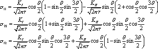

![]()
while the displacements can be calculated by integrating the strains, with the result
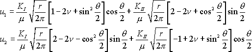
![]()


![]()
Note that this displacement field is valid for plane strain deformation only.
Observe that the stress intensity factor has the
bizarre units of ![]()
![]()
![]()
![]()
![]() .
.
The assumptions of phenomenological linear elastic fracture mechanics
The objective of linear elastic fracture mechanics is to predict the critical loads that will cause a crack in a solid to grow. For fatigue applications or dynamic fracture, the rate and direction of crack growth are also of interest.
The phenomenological theory is based on the following loose argument. Consider a crack in a reasonably brittle, isotropic solid. If the solid were ideally elastic, we would expect the asymptotic solution listed in the preceding section to become progressively more accurate as we approach the crack tip. Away from the crack tip, the fields are influenced by the geometry of the solid and boundary conditions, and the asymptotic crack tip field would not be accurate. In practice, the asymptotic field will also not give an accurate representation of the stress fields very close to the crack tip either. The crack may not be perfectly sharp at its tip, and if it were, no solid could withstand the infinite stress predicted by our asymptotic linear elastic solution. We therefore anticipate that in practice the linear elastic solution will not be accurate very close to the crack tip itself, where material nonlinearity and other effects play an important role. So the true stress and strain distributions will have 3 general regions
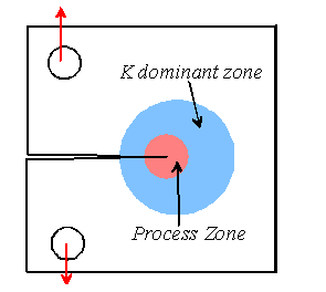
1. Close to the crack tip, there will be a process zone, where the material suffers irreversible damage.
2. A bit further from the crack tip, there will be a region where the linear elastic field asymptotic crack tip field might be expected to be accurate. This is known as the `region of K dominance
3. Far from the crack tip the stress field depends on the geometry of the solid and boundary conditions.
Material failure (crack growth or fatigue) is a
consequence of the ugly stuff that goes on in the process zone. Linear
elastic fracture mechanics postulates that one doesnt need to understand this
ugly stuff in detail, since the fields in the process zone are likely to be
controlled mainly by the fields in the region of K dominance. The fields
in this region depend only on the three stress intensity factors ![]()
![]()
![]()
![]()
![]() .
Therefore, the state in the process zone can be characterized for
phenomenological purposes by the three stress intensity factors.
.
Therefore, the state in the process zone can be characterized for
phenomenological purposes by the three stress intensity factors.
If this is true, the conditions for crack growth, or
the rate of crack growth, will be only a function of stress intensity factor
and nothing else. We can measure the critical value of ![]()
![]()
![]()
![]()
![]() required
to cause the crack to grow in a standard laboratory test, and use this as a
measure of the resistance of the solid to crack propagation. For fatigue
tests, we can measure crack growth rate as a function of
required
to cause the crack to grow in a standard laboratory test, and use this as a
measure of the resistance of the solid to crack propagation. For fatigue
tests, we can measure crack growth rate as a function of ![]()
![]()
![]()
![]()
![]() or
its history, and characterize the relationship using appropriate phenomenological
laws.
or
its history, and characterize the relationship using appropriate phenomenological
laws.
Having characterized the material, we can then estimate the safety of a structure or component that containing a crack. To do so, calculate the stress intensity factors for the crack in the structure, and then use our phenomenological fracture or fatigue laws to decide whether or not the crack will grow.
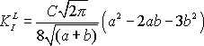
For example, the fracture criterion under mode I loading is written
![]()
![]()
![]()
![]()
![]()
for crack growth, where ![]()
![]()
![]()
![]()
![]() is
the critical stress intensity factor for the onset of fracture. The
critical stress intensity factor is referred to as the fracture toughness
of the solid.
is
the critical stress intensity factor for the onset of fracture. The
critical stress intensity factor is referred to as the fracture toughness
of the solid.
Empirically, it is found that this approach works quite well, provided that the assumptions inherent in linear elastic fracture mechanics are satisfied.
Careful tests have established the following standards for the applicability of linear elastic fracture mechanics.
1. All characteristic specimen dimensions must exceed 25 times the expected plastic zone size at the crack tip
2. For plane strain conditions at the crack tip the specimen thickness must exceed at least the plastic zone size.
For a material with yield stress Y
loaded in Mode I with stress intensity factor ![]()
![]()
![]()
![]()
![]() the
plastic zone size can be estimated as
the
plastic zone size can be estimated as

![]()
![]()
![]()
![]()
Practical application of linear elastic fracture mechanics
To apply LEFM in a design application, you need to be able to do three things.
1. Measure the critical stress intensity factors that cause fracture in your material, or measure fatigue crack growth rates as a function of static or cyclic stress intensity
2. Estimate the anticipated size and location of cracks in your structure or component
3. Calculate the stress intensity factors for the cracks in your structure or component under anticipated loading conditions.
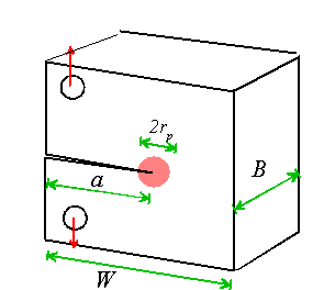
A. Fracture toughness measurements
For structural applications, standard testing techniques are available to measure material properties for fracture applications. Two standard test specimen geometries are shown below

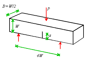
(a) Compact tension specimen (b) 3 point bend specimen
Stress intensity factors for these specimens have been carefully computed as a function of crack length and the results fit by curves
Compact tension specimen:

![]()
![]()
![]()
![]()
Three point bend specimen.

![]()
![]()
![]()
![]()
Various other test specimens exist.
Conducting a fracture test or fatigue test is (at least conceptually) straightforward you make a specimen (for fracture tests a sharp crack is usually created by initiating a fatigue crack at the tip of a notch); and load it in a tensile testing machine.
For a fracture test, you measure the critical
load when the crack starts to grow. It can be difficult to detect the
onset of crack growth. For this reason, the usual approach is to monitor
the crack opening displacement ![]()
![]()
![]()
![]()
![]() during
the test, then plot load as a function of crack opening displacement. A
typical result is illustrated below.
during
the test, then plot load as a function of crack opening displacement. A
typical result is illustrated below.
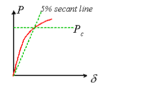
The load-CTOD curve ceases to be linear when the
crack begins to grow. This point is hard to identify, so instead the
convention is to draw a line with slope 5% lower than the initial ![]()
![]()
![]()
![]()
![]() curve
(the 5% secant line) and use the point where this line intersects the
curve
(the 5% secant line) and use the point where this line intersects the ![]()
![]()
![]()
![]()
![]() as
the fracture load. The plane strain fracture toughness of the material,
as
the fracture load. The plane strain fracture toughness of the material, ![]()
![]()
![]()
![]()
![]() , is
deduced from the fracture load, using the calibration for the specimen.
, is
deduced from the fracture load, using the calibration for the specimen.
After measurement, one must check that ![]()
![]()
![]()
![]()
![]() is
within the limits required for K dominance in the specimen, following the rules
in the preceding section.
is
within the limits required for K dominance in the specimen, following the rules
in the preceding section.
A few typical values of fracture toughness are tabulated below.
|
Material |
Approximate fracture toughness, |
|
Mild steel |
140 |
|
High carbon steel |
30 |
|
Nickel, copper |
>100 |
|
Aluminum and alloys |
1--50 |
|
Alumina |
3-5 |
|
Glasses, rocks |
1 |
|
Concrete |
0.2 |
Stable Tearing Kr curves and Crack Stability
In ideally brittle materials, fracture is a catastrophic event. Once the load reaches the level required to trigger crack growth, the crack continues to propagate dynamically through the specimen. In more ductile materials, a period of stable crack growth under steadily increasing load may occur prior to complete failure. This behavior is particularly common in tearing of thin sheets of metals, but stable crack growth is observed in most materials even polycrystalline ceramics.
Stable crack growth in metals usually occurs because a zone of plastically deformed material is left in the wake of the crack. This deformed material tends to reduce the stresses at the crack tip. In brittle polycrystalline ceramics, or in fiber reinforced brittle composites, the stable crack growth is caused by the formation of a `bridging zone behind the crack tip. Some fibers, or grains, remain intact in the crack wake, and tend to hold the crack faces shut, increasing the apparent strength of the solid.
In some materials, the increase in load during
stable crack growth is so significant that its worth accounting for the effect
in design calculations. The protective effect of the process zone in the
crack wake is modeled phenomenologically, by making the toughness of the
material a function of the increase in crack length. The apparent
toughness is measured in the same way as ![]()
![]()
![]()
![]()
![]() -
a pre-cracked specimen is subjected to progressively increasing load, and the
crack length is monitored either optically or using compliance methods (more on
this later). A value of
-
a pre-cracked specimen is subjected to progressively increasing load, and the
crack length is monitored either optically or using compliance methods (more on
this later). A value of ![]()
![]()
![]()
![]()
![]() can
be computed for the specimen using the calibrations during crack growth it is
assumed that
can
be computed for the specimen using the calibrations during crack growth it is
assumed that ![]()
![]()
![]()
![]()
![]() is
equal to the fracture toughness of the material.
is
equal to the fracture toughness of the material.
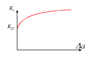
The results are plotted in a `resistance curve or
`R curve for the material. The fracture toughness ![]()
![]()
![]()
![]()
![]() is
the critical stress intensity factor required to initiate crack growth.
The variation of stress intensity factor with crack growth is denoted
is
the critical stress intensity factor required to initiate crack growth.
The variation of stress intensity factor with crack growth is denoted ![]()
![]()
![]()
![]()
![]() .
.
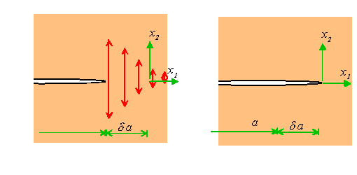
The resistance curve is then used to predict the
conditions necessary for unstable crack growth through the material. To
see how this is done, consider a large sample of material containing a slit
crack of length 2a, subjected to stress ![]()
![]()
![]()
![]()
![]() .
The stress intensity factor (from the table) is
.
The stress intensity factor (from the table) is ![]()
![]()
![]()
![]()
![]() .
Crack growth begins when
.
Crack growth begins when ![]()
![]()
![]()
![]()
![]() .
Thereafter, there will be a period of stable crack growth, during which the
applied stress increases. The stress satisfies
.
Thereafter, there will be a period of stable crack growth, during which the
applied stress increases. The stress satisfies
![]()
![]()
![]()
![]()
![]()
The stress will continue to increase as long as the increase in toughness with crack length is sufficient to overcome the increase in stress intensity factor with crack length. Catastrophic failure (unstable crack growth ) will occur when continued crack growth is possible at constant or decreasing load. This requires
![]()
![]()
![]()
![]()
![]()
For the case of a slit crack, this gives
![]()
![]()
![]()
![]()
![]()
for the critical stress at unstable fracture.
Mixed Mode fracture criteria
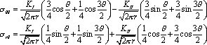
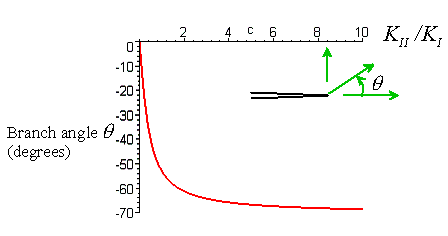
Fracture toughness is almost always measured under mode I loading (except when measuring fracture toughness of a bi-material interface). If a crack is subjected to combined mode I and mode II loading, a mixed mode fracture criterion is required. There are several ways to construct mixed mode fracture criteria the issue has been the subject of some quite heated arguments. The criterion of maximum hoop stress is one example. Recall that the crack tip hoop and shear stresses are

![]()

![]()
The maximum hoop stress criterion postulates that a
crack under mixed mode loading starts to propagate when the greatest value of
hoop stress ![]()
![]()
![]()
![]()
![]() reaches
a critical magnitude, at which point the crack will branch at the angle for
which
reaches
a critical magnitude, at which point the crack will branch at the angle for
which ![]()
![]()
![]()
![]()
![]() is
greatest (or equivalently the angle for which
is
greatest (or equivalently the angle for which ![]()
![]()
![]()
![]()
![]() ).
The critical angle is plotted as a function of
).
The critical angle is plotted as a function of ![]()
![]()
![]()
![]()
![]() below.
The asymptote for
below.
The asymptote for ![]()
![]()
![]()
![]()
![]() is
70.7 degrees.
is
70.7 degrees.
The failure locus predicted by this criterion is shown below
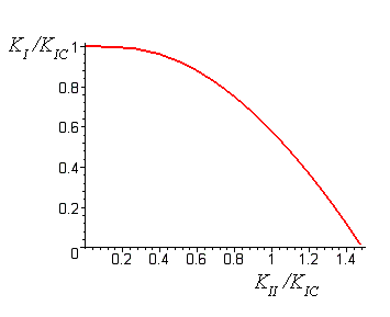
All available criteria predict that, after branching, a crack will follow a path such that the local mode II stress intensity factor vanishes.
Fatigue testing
For a fatigue test, the crack length is measured (optically, or using compliance techniques) as a function of time or number of load cycles. Fatigue laws are deduced by plotting crack growth rate as a function of applied stress intensity factor. Typical static fatigue data (e.g. for corrosion crack growth, or creep crack growth) show behavior shown below
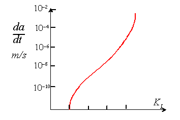
Most materials have a fatigue threshold a
value of ![]()
![]()
![]()
![]()
![]() below
which crack growth is undetectable. Then there is a range where crack
growth rate shows a power-law dependence on stress intensity factor of the form
below
which crack growth is undetectable. Then there is a range where crack
growth rate shows a power-law dependence on stress intensity factor of the form
![]()
![]()
![]()
![]()
![]()
where m is typically
of order 5-10. Finally, for values of ![]()
![]()
![]()
![]()
![]() approaching
the fracture toughness, the crack growth rate increases drastically with
approaching
the fracture toughness, the crack growth rate increases drastically with ![]()
![]()
![]()
![]()
![]() .
.
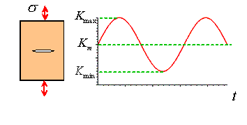
Under cyclic loading, the crack is subjected to a cycle of mode I and mode II stress intensity factor. Most fatigue tests are performed under a steady cycle of pure mode I loading, as sketched below.
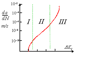
The results are usually displayed by plotting the crack growth per cycle as a function of the stress intensity factor range
![]()
![]()
![]()
![]()
![]()
A typical result shows three regions. There is a
fatigue threshold ![]()
![]()
![]()
![]()
![]() below
which crack growth is undetectable. For modest loads, the crack growth
rate obeys
below
which crack growth is undetectable. For modest loads, the crack growth
rate obeys
![]()
![]()
![]()
![]()
![]()
where the index n is between 2 and 4. As the maximum stress intensity factor approaches the fracture toughness of the material, the crack growth rate accelerates dramatically.
In the Paris law regime, the crack growth rate is
not sensitive to the mean value of stress intensity factor ![]()
![]()
![]()
![]()
![]() .
In the other two regimes,
.
In the other two regimes, ![]()
![]()
![]()
![]()
![]() has
a noticeable effect - the fatigue threshold is reduced as
has
a noticeable effect - the fatigue threshold is reduced as ![]()
![]()
![]()
![]()
![]() increases,
and the crack growth rate in regime III increases with
increases,
and the crack growth rate in regime III increases with ![]()
![]()
![]()
![]()
![]() .
.
B. Finding cracks in structures
This is always the weak link in fracture mechanics. For most practical applications you simply dont know if your component will have a crack in it, and it will cost you big-time if you need to find out. Your options are:
1. Take a wild guess, based on microscopic examinations of representative samples of material. Alternatively, you can specify the biggest flaw you are prepared to tolerate and insist that your materials processing slaves manufacture appropriately defect free materials.
2. Conduct a proof test (popular e.g. with pressure vessel applications) wherein the structure or component is subjected to a load greatly exceeding the anticipated service load under controlled conditions. If the fracture toughness of the material is known, you can then deduce the largest crack size that could be present in the structure without causing failure during proof testing.
3. Use some kind of non-destructive test technique to attempt to detect cracks in your structure. Examples of such techniques are ultrasound, where you look for echoes off crack surfaces; x-ray techniques; and inspection with optical microscopy. If you detect a crack, most of these techniques will allow you to estimate the crack length. If not, you have to assume for design purposes that your structure is loaded with cracks that are just too short to be detected.
C. Calculating stress intensity factors
Various techniques can be used to calculate stress intensity factors, including
1. Solve the full linear elastic boundary value problem, and deduce stress intensities from the asymptotic behavior of the stress field near the crack tips
2. Attempt to deduce stress intensity factors directly using energy methods or path independent integrals
3. Look up the solution you need in tables
4. Use a numerical method boundary integral equation methods are particularly effective for crack problems, but FEM can be used too.
Analytical solutions to some crack problems
Calculating stress intensity factors for a crack in a structure or component involves the solution of a standard linear elastic boundary value problem. Once the stresses have been computed, the stress intensity factor is deduced from the definitions
![]()
![]()
![]()
![]()
![]()
![]()
![]()
![]()
![]()
![]()
Note that stress components must be expressed in a basis oriented correctly with respect to the crack tip when taking this limit.
Exact solutions are known for a few simple geometries. A couple of examples are
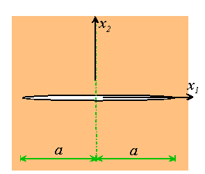
2D Slit crack in an infinite solid
The displacement field for the anti-plane shear problem can be computed from the complex potential
![]()
![]()
![]()
![]()
![]()
and the mode III stress intensity factor follows as
![]()
![]()
![]()
![]()
![]()
The solution to the equivalent plane strain problem can be generated by complex potentials
![]()
![]()
![]()
![]()
and the mode I and mode II stress intensity factors can be computed as
![]()
![]()
![]()
![]()
![]()
Some care is required to evaluate the square root in the complex potentials properly (they are multiple valued and you need to put the branch cut in the right place). For this purpose, it is helpful to note that the appropriate branch can be obtained by setting
![]()
![]()
![]()
![]()
![]()
with ![]()
![]()
![]()
![]()
![]()
Penny shaped crack in an infinite solid
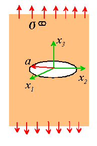
This problem was discussed in some detail in Section 6.1. Displacement and stress fields are generated by superposing the uniform stress state

![]()
![]()
![]()
![]()
with a corrective solution derived from a harmonic potential
![]()
![]()
![]()
![]()
![]()
where ![]()
![]()
![]()
![]()
![]() ,
and stresses and displacement are computed using the half-plane representation
for elastostatic states introduced in Sect. 4
,
and stresses and displacement are computed using the half-plane representation
for elastostatic states introduced in Sect. 4
![]()
![]()
![]()
![]()
![]()
![]()
![]()
![]()
![]()
![]()
The best way to use this expression is to evaluate the appropriate derivatives under the integral defining the potential, in which case the integral can be evaluated in closed form (at least on the plane of the crack). The stress intensity factor follows as
![]()
![]()
![]()
![]()
![]()
It is not always necessary to solve the full linear elastic boundary value problem in order to compute stress intensity factors. Energy methods, or the application of path independent integrals, can sometimes be used to obtain stress intensity factors directly. This will be discussed in more detail below.
Vast numbers of crack problems have been solved to catalog stress intensity factors in various geometries of interest. Two excellent (but expensive) sources of such solutions are Tadas Handbook of Stress Intensity Factors, and Murakamis 3 volume set of stress intensity factor tables. A few important (and relatively simple) results are listed below.
A short table of stress intensity factors
2D Slit crack in an infinite solid
![]()
![]()
![]()
![]()
![]()
3D circular crack in an infinite solid under remote tension
![]()
![]()
![]()
![]()
![]()
Line loads acting on the faces of a semi-infinite crack
![]()
![]()
![]()
![]()
![]()
Line forces acting on the faces of a slit crack
![]()
![]()
![]()
![]()
![]()
(these are for the right hand crack tip)
Edge crack in a half-plane
![]()
![]()
![]()
![]()
![]()
Point forces acting on the faces of a semi-infinite crack
![]()
![]()
![]()
![]()
![]()
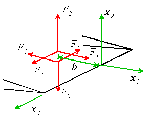
The Bueckner superposition
The point force solutions are particularly useful, because they allow you to calculate stress intensity factors for a crack in an arbitrary stress field using a simple superposition argument. The procedure works like this. We start by computing the stress field in a solid without a crack in it. This solution satisfies all boundary conditions except that the crack faces are subject to tractions. We could correct solution by applying pressure (and shear) to the crack faces that are just sufficient to remove the unwanted tractions. If we know the stress intensity factors induced by point forces acting on the crack faces, we can use superpose this solution to calculate stress intensity factors induced by the corrective pressure distribution.
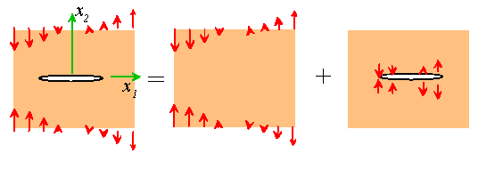
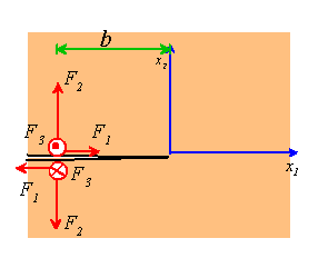
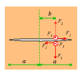
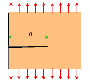
As an example, suppose that we want to calculate stress intensity factors for a crack in a bending stress field, as illustrated in the figure above.
In the uncracked solid, the normal traction acting along the line of the crack is
![]()
![]()
![]()
![]()
![]()
where C is the stress gradient. As a first approximateion we remove the tractions from the entire crack by applying pressure to the crack faces, which (from the tables above) induces stress intensity factors

![]()
![]()
![]()
![]()
at the left and right crack tips. Evaluating the integrals gives
![]()
![]()
![]()
![]()
![]()
Note that the stress intensity factor at the left crack tip is predicted to be negative. This cannot be correct from the asymptotic stress field we know that if the stress intensity factor is negative, the crack faces must overlap behind the crack tip (the displacement jump is negative).
With a bit of cunning, we can fix this
problem. The cause of the error in the quick estimate is that we removed
tractions from the entire crack this was a mistake; we should only have
removed tractions from parts of the crack faces that open up. So
lets suppose that the crack closes at ![]()
![]()
![]()
![]()
![]() ,
and put the left hand crack tip there. The stress intensity factors are
then
,
and put the left hand crack tip there. The stress intensity factors are
then

![]()
![]()
![]()
![]()
This gives
![]()
![]()
![]()
![]()
for the stress intensity
factor at the left hand crack tip. The stress must be bounded at ![]()
![]()
![]()
![]()
![]() where
the crack faces touch, so that
where
the crack faces touch, so that ![]()
![]()
![]()
![]()
![]() .
This gives
.
This gives ![]()
![]()
![]()
![]()
![]() .
The stress intensity factor at the right hand crack tip then follows as
.
The stress intensity factor at the right hand crack tip then follows as
![]()
![]()
![]()
![]()
![]()
![]()
![]()
![]()
![]()
![]()
This is not very different to our earlier estimate. This illustrates a general feature of the field of fracture mechanics. There are many opportunities to do clever things, but often the results of all the cleverness are pretty useless.
Energy approach to fracture
Energy methods provide a very powerful approach to crack problems.
Energy release rate
Consider an ideally elastic solid with elastic
constants ![]()
![]()
![]()
![]()
![]() subjected
to some loading (applied tractions, displacements, or body forces).
Suppose the solid contains a crack, with length a. Define the
potential energy of the solid in the usual way as
subjected
to some loading (applied tractions, displacements, or body forces).
Suppose the solid contains a crack, with length a. Define the
potential energy of the solid in the usual way as
![]()
![]()
![]()
![]()
![]()
Let the crack increase in size, so that at a
position s on the crack front, the crack advances by ![]()
![]()
![]()
![]()
![]() with
loading kept fixed. The principle of minimum potential energy (sect 4)
shows that
with
loading kept fixed. The principle of minimum potential energy (sect 4)
shows that ![]()
![]()
![]()
![]()
![]() ,
since the displacement field associated with
,
since the displacement field associated with ![]()
![]()
![]()
![]()
![]() is
a kinematically admissible field for the solid with a longer crack. The energy
release rate
is
a kinematically admissible field for the solid with a longer crack. The energy
release rate ![]()
![]()
![]()
![]()
![]() around
the crack front is defined so that
around
the crack front is defined so that
![]()
![]()
![]()
![]()
![]()
Energy release rate has units of ![]()
![]()
![]()
![]()
![]() (energy
per unit area)
(energy
per unit area)
Energy release rate as a fracture criterion
Phenomenological fracture (or fatigue) criteria can be based on energy release rate arguments as an alternative to the K based fracture criteria discussed earlier.
The argument is as follows. Regardless of the actual mechanisms involved, crack propagation involves dissipation (or conversion) of energy. A small amount of energy is required to create two new free surfaces (twice the surface energy per unit area of crack advance, to be precise). In addition, there may be a complex process zone at the crack tip, where the material is plastically deformed; voids may be nucleated; there may be chemical reactions; and generally all hell breaks loose. All these processes involve dissipation of energy. We postulate, however, that the process zone remains self-similar during crack growth. If this is the case, energy will be dissipated at a constant rate during crack growth. The crack can only grow if the rate of change of potential energy is sufficient to provide this energy.
This leads to a fracture criterion of the form
![]()
![]()
![]()
![]()
![]()
for crack growth, where ![]()
![]()
![]()
![]()
![]() is
a property of the material. Unfortunately
is
a property of the material. Unfortunately ![]()
![]()
![]()
![]()
![]() is
often referred to as the fracture toughness of a solid, just like
is
often referred to as the fracture toughness of a solid, just like ![]()
![]()
![]()
![]()
![]() defined
earlier. It is usually obvious from dimensional considerations which one
is being used, but its an annoying source of
confusion.
defined
earlier. It is usually obvious from dimensional considerations which one
is being used, but its an annoying source of
confusion.
Relation between energy release rate and stress intensity factor
Of course, G is closely related to K. A neat argument due to Irwin provides the connection.
A crack of length a can be regarded as a
crack with ![]()
![]()
![]()
![]()
![]() which
is being pinched by an appropriate distribution of traction acting on the crack
faces between
which
is being pinched by an appropriate distribution of traction acting on the crack
faces between ![]()
![]()
![]()
![]()
![]() and
and
![]()
![]()
![]()
![]()
![]() .
We can therefore calculate the change in potential energy as the crack
propagates by distance
.
We can therefore calculate the change in potential energy as the crack
propagates by distance ![]()
![]()
![]()
![]()
![]() by
computing the work done as these tractions are progressively relaxed to
zero.
by
computing the work done as these tractions are progressively relaxed to
zero.
The asymptotic crack tip field gives the tractions acting on the upper crack face as
![]()
![]()
![]()
![]()
![]()
(equal and opposite tractions must act on the lower crack face). As the crack is allowed to open, the upper crack face displaces by
![]()
![]()
![]()
![]()
![]()
where we have assumed plane strain deformation. The total work done as the tractions are relaxed quasi-statically to zero is
![]()
![]()
![]()
![]()
![]()
(the work done by tractions acting on the upper
crack face per unit length is ![]()
![]()
![]()
![]()
![]() ,
and there are two crack faces). Evaluating the integrals gives
,
and there are two crack faces). Evaluating the integrals gives
![]()
![]()
![]()
![]()
![]()
The same result can be obtained by applying crack tip energy flux integrals, to be discussed shortly.
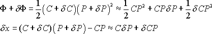
Relation between energy release rate and compliance
Energy release rate is related to the compliance of
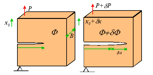
a structure or specimen. Consider the compact tension specimen shown in
the picture. Suppose that the specimen is subjected to a load P,
which causes the point of application of the load to displace by a distance ![]()
![]()
![]()
![]()
![]() in
a direction parallel to the load. The compliance of the specimen would be
in
a direction parallel to the load. The compliance of the specimen would be
![]()
![]()
![]()
![]()
![]()
The load induces a total strain energy ![]()
![]()
![]()
![]()
![]() in
the specimen.
in
the specimen.
Now, suppose that the crack extends by a distance ![]()
![]()
![]()
![]()
![]() .
During crack growth, the load increases to
.
During crack growth, the load increases to ![]()
![]()
![]()
![]()
![]() and
displaces to
and
displaces to ![]()
![]()
![]()
![]()
![]() .
In addition, the strain energy changes to
.
In addition, the strain energy changes to ![]()
![]()
![]()
![]()
![]() ,
while the compliance increases to
,
while the compliance increases to ![]()
![]()
![]()
![]()
![]() .
The energy released during crack advance is the change in strain energy, less
the work done by applied loads, so that
.
The energy released during crack advance is the change in strain energy, less
the work done by applied loads, so that
![]()
![]()
![]()
![]()
![]()
Note that
![]()
![]()
![]()
![]()
whence
![]()
![]()
![]()
![]()
![]()
The energy release rate therefore is related to compliance by
![]()
![]()
![]()
![]()
![]()
This result is useful for several reasons. Firstly, it can sometimes be used to calculate energy release rates, and possibly also deduce stress intensity factors, for structures whose rate of change of compliance with crack length can be easily determined. One example is the cantilever beam specimen shown below
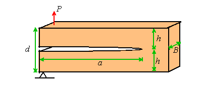
The deflection d of the load must be twice that of a cantilever beam, length a, width B and height h, encastre on its right hand end and subjected to a load P at its left hand end. From elementary strength of materials theory
![]()
![]()
![]()
![]()
![]()
where E is the Youngs modulus of the specimen. Thus
![]()
![]()
![]()
![]()
![]()
The energy release rate therefore follows as
![]()
![]()
![]()
![]()
![]()
By symmetry, the crack must be loaded in pure mode I. We can therefore deduce the stress intensity factor using the relation
![]()
![]()
![]()
![]()
![]()
and recalling that ![]()
![]()
![]()
![]()
![]() we
obtain
we
obtain
![]()
![]()
![]()
![]()
![]()
The J integral and other crack tip integrals
One of the most common tasks in the application of fracture mechanics is to determine crack tip quantities (energy release rate, or stress intensity factor) in terms of boundary loading. Path independent integrals provide a way to do this. They have many other applications besides a particularly important one is that they provide crucial insight into the nature of crack tip fields in nonlinear elastic or plastic solids, and therefore provide a tool for analyzing fracture in fully plastic solids.
As a starting point we set out to devise an
alternative way to compute the energy release rate for a crack, which applies
not only to linear elastic solids under quasi-static loading conditions, but is
completely independent of the constitutive response of the solid, and also
applies under dynamic loading (it is restricted to small strains,
however). The approach will be to find an expression for the flux of
energy through a cylindrical surface ![]()
![]()
![]()
![]()
![]() enclosing
the crack tip, which moves with the crack. We will get the energy release
rate by shrinking the surface down onto the crack tip.
enclosing
the crack tip, which moves with the crack. We will get the energy release
rate by shrinking the surface down onto the crack tip.
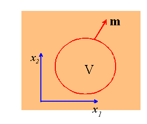
To proceed, we need a general expression for the
energy flux across a surface in a solid. Consider an arbitrary surface S
in a solid enclosing some volume V. The surface need not
necessarily be a material surface it could move with respect to the
solid. Let ![]()
![]()
![]()
![]()
![]() denote
the displacement, (infinitesimal) strain and stress field in the solid, and let
denote
the displacement, (infinitesimal) strain and stress field in the solid, and let
![]()
![]()
![]()
![]()
![]() denote
the velocity of a material point with respect to a fixed origin. Assume
that the solid is free of body forces, for simplicity. The rate of change
of mechanical energy density at a point inside V follows as
denote
the velocity of a material point with respect to a fixed origin. Assume
that the solid is free of body forces, for simplicity. The rate of change
of mechanical energy density at a point inside V follows as
![]()
![]()
![]()
![]()
![]()
where ![]()
![]()
![]()
![]()
![]() is
the stress power density and
is
the stress power density and ![]()
![]()
![]()
![]()
![]() is
the kinetic energy density. Define the work flux vector
is
the kinetic energy density. Define the work flux vector ![]()
![]()
![]()
![]()
![]() .
Then
.
Then
![]()
![]()
![]()
![]()
![]()
To see this, substitute for work flux vector and mechanical energy density in terms of stress and displacement to get
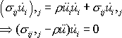
![]()
![]()
![]()
![]()
which is evidently satisfied for any stress field and acceleration field related through the linear momentum balance equation. Now, integrate over the volume V and apply the divergence theorem to see that
![]()
![]()
![]()
![]()
![]()
Finally, apply the Reynolds transport theorem to the term on the right hand side

![]()
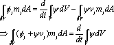

![]()
where ![]()
![]()
![]()
![]()
![]() denotes
the velocity of the surface
denotes
the velocity of the surface ![]()
![]()
![]()
![]()
![]() .
The term on the right hand side clearly represents the total rate of change of
mechanical energy in V. Consequently, the term on the left hand
side must represent the mechanical energy flux across
.
The term on the right hand side clearly represents the total rate of change of
mechanical energy in V. Consequently, the term on the left hand
side must represent the mechanical energy flux across ![]()
![]()
![]()
![]()
![]() .
This is the result we need.
.
This is the result we need.
We can use this result to obtain an expression for
the energy flux to a crack tip. Suppose the crack tip runs with steady
speed v in the ![]()
![]()
![]()
![]()
![]() direction.
Let
direction.
Let ![]()
![]()
![]()
![]()
![]() denote
a cylindrical surface enclosing the crack tip, which moves with the crack
tip. The energy flux through
denote
a cylindrical surface enclosing the crack tip, which moves with the crack
tip. The energy flux through ![]()
![]()
![]()
![]()
![]() follows
as
follows
as
![]()
![]()
![]()
![]()
![]()
where ![]()
![]()
![]()
![]()
![]() is
the kinetic energy and
is
the kinetic energy and ![]()
![]()
![]()
![]()
![]() is
the stress work. The energy flux to the crack tip follows by taking the
limit as
is
the stress work. The energy flux to the crack tip follows by taking the
limit as ![]()
![]()
![]()
![]()
![]() shrinks
down onto the crack tip.
shrinks
down onto the crack tip.
To obtain an expression for the energy release rate,
assume that the crack tip fields remain self-similar (i.e. an observer
traveling with the crack tip sees a fixed state of strain and stress). In
addition, assume that the crack front is straight, and has length L in
direction perpendicular to the plane of the figure. Under these
conditions ![]()
![]()
![]()
![]()
![]() ,
and
,
and ![]()
![]()
![]()
![]()
![]() .
Consequently
.
Consequently
![]()
![]()
![]()
![]()
![]()
where C is a contour enclosing the crack tip. (Equivalent results can be derived for general 3D cracks, but these details are omitted here).
This result is valid for any material response, and applies to both static and dynamic conditions. The result becomes particularly useful if we make two further assumptions:
(1) Quasi-static loading
(2) The material is elastic (but not necessarily linear elastic)
In this case W is the strain energy density
of the material for a linear elastic solid ![]()
![]()
![]()
![]()
![]() .
.
With these assumptions, it turns out that the crack tip energy integral is path independent. There is no need then to shrink the contour down onto the crack tip we get the same answer for any contour that encloses the crack tip.
To see this, evaluate the integral defining G
around any closed contour ![]()
![]()
![]()
![]()
![]() ,
and apply the divergence theorem
,
and apply the divergence theorem
![]()
![]()
![]()
![]()
![]()
where A is the area enclosed by ![]()
![]()
![]()
![]()
![]() and
we have noted that
and
we have noted that
![]()

![]()
Now, evaluate the integral around the closed contour shown below
Note that the integrand vanishes on ![]()
![]()
![]()
![]()
![]() and
and
![]()
![]()
![]()
![]()
![]() so
that
so
that
![]()
![]()
![]()
![]()
![]()
Now reverse the direction of integration around ![]()
![]()
![]()
![]()
![]() (note
that m = -n) to get
(note
that m = -n) to get
![]()
![]()
![]()
![]()
![]()
giving path in dependence as required.
This result is exploited by defining the J integral
![]()
![]()
![]()
![]()
![]()
When evaluated around the tip of a stationary crack in an elastic material, J is path independent. In addition J=G under these conditions, giving a way to compute energy release rates.
The J integral has many applications.
In some cases it can be used to compute energy release rates. For
example, consider the problem shown below. A long linear elastic cracked
strip is clamped between rigid boundaries. The bottom boundary is held
fixed; the top is displaced vertically by a distance ![]()
![]()
![]()
![]()
![]() .
Calculate the energy release rate for the crack.
.
Calculate the energy release rate for the crack.
For this case J=G and we can easily evaluate
the J integral around the contour shown. The integrand vanishes
everywhere except the segment ![]()
![]()
![]()
![]()
![]() .
On this segment it is easy to see that
.
On this segment it is easy to see that

![]()
![]()
![]()
![]()
while ![]()
![]()
![]()
![]()
![]() can
be made arbitrarily small by taking
can
be made arbitrarily small by taking ![]()
![]()
![]()
![]()
![]() far
ahead of the crack tip. Therefore, evaluating the integral, we get
far
ahead of the crack tip. Therefore, evaluating the integral, we get

![]()
![]()
![]()
![]()
Symmetry conditions show that the crack must be loaded in pure mode I, so the stress intensity factor can also be computed.
Cracks in elastic-plastic materials
Thus far we have shied away from the obscene stuff that goes on in the process zone near the crack tip. (The mention of obscene stuff will probably increase the hit-rate to this website!) . But we cant avoid this indefinitely. To know the limitations of LEFM, we need some way to estimate the plastic zone size at the crack tip, at the very least. The stress and strain fields inside the plastic zone are also of some interest.
Dugdale-Barenblatt cohesive zone model of yield at a crack tip
The simplest estimate of plastic zone size can be
obtained using Dugdale & Barenblatts cohesive zone model. Consider a
crack of length 2a in an elastic-perfectly plastic material with elastic
constants ![]()
![]()
![]()
![]()
![]() and
yield stress Y. We anticipate that there will be a region near
each crack tip where the material deforms plastically. The Mises
equivalent stress
and
yield stress Y. We anticipate that there will be a region near
each crack tip where the material deforms plastically. The Mises
equivalent stress ![]()
![]()
![]()
![]()
![]() should
not exceed yield in this region. Its hard to find a solution with
stresses at yield everywhere in the plastic zone, but we can easily construct
an approximate solution where the stress along the line of the crack satisfies
the yield condition, using a cohesive zone model.
should
not exceed yield in this region. Its hard to find a solution with
stresses at yield everywhere in the plastic zone, but we can easily construct
an approximate solution where the stress along the line of the crack satisfies
the yield condition, using a cohesive zone model.

Let ![]()
![]()
![]()
![]()
![]() denote
the length of the cohesive zone at each crack tip. To construct an
appropriate solution we extend the crack in both directions to put fictitious
crack tips at
denote
the length of the cohesive zone at each crack tip. To construct an
appropriate solution we extend the crack in both directions to put fictitious
crack tips at ![]()
![]()
![]()
![]()
![]() ,
and distribute tractions of magnitude
,
and distribute tractions of magnitude ![]()
![]()
![]()
![]()
![]() over
the crack flanks from
over
the crack flanks from ![]()
![]()
![]()
![]()
![]() to
to
![]()
![]()
![]()
![]()
![]() ,
and similarly at the other crack tip.. Evidently, the stress then
satisfies
,
and similarly at the other crack tip.. Evidently, the stress then
satisfies ![]()
![]()
![]()
![]()
![]() along
the line of the crack just ahead of each crack.
along
the line of the crack just ahead of each crack.
We can use our point force solution to compute the stress intensity factor at the fictitious crack tip. Omitting the tedious details of evaluating the integral, we find that
![]()
![]()
![]()
![]()
![]()
The * on the stress intensity factor is introduced
to emphasize that this is not the true crack tip stress intensity factor (which
is of course ![]()
![]()
![]()
![]()
![]() ),
but the stress intensity factor at the fictitious crack tip. The stresses must
remain bounded just ahead of the fictitious crack tip, so that
),
but the stress intensity factor at the fictitious crack tip. The stresses must
remain bounded just ahead of the fictitious crack tip, so that ![]()
![]()
![]()
![]()
![]() must
be chosen to satisfy
must
be chosen to satisfy ![]()
![]()
![]()
![]()
![]() .
This gives
.
This gives

![]()
![]()
![]()
![]()
Its more sensible to express this in terms of stress intensity factor

![]()
![]()
![]()
![]()
This estimate turns out to be remarkably accurate for plane stress conditions, where the `official plastic zone size is

![]()
![]()
![]()
![]()
For plane strain the plastic zone is smaller, the official plastic zone size is
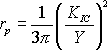
![]()
![]()
![]()
![]()
Hutchinson-Rice-Rosengren crack tip fields for stationary crack in a power law hardening solid
The cohesive zone model gives a quick and dirty estimate of plastic zone size but its not an accurate solution to the stress and strain fields near a crack tip in a plastically deforming material.
The famous HRR crack tip field gives a more accurate
picture. The HRR field is derived in a similar way to the asymptotic
elastic solution described earlier. We (actually HRR, not us) consider an
infinite solid containing an infinitely long crack aligned with front along the
![]()
![]()
![]()
![]()
![]() axis.
The crack tip is stationary, and the solid is subjected to remote loading. To
make progress, the solid is idealized not as a plastic solid, but instead using
the deformation theory of plasticity (i.e. as a hypoelastic
solid). Once we have the solution, it turns out that material elements
near the crack tip experience a proportional cycle of stress and strain as the
remote load is increased. Consequently the deformation plasticity model
provides an exact solution for a rigid plastic Mises solid with pure power law
hardening.
axis.
The crack tip is stationary, and the solid is subjected to remote loading. To
make progress, the solid is idealized not as a plastic solid, but instead using
the deformation theory of plasticity (i.e. as a hypoelastic
solid). Once we have the solution, it turns out that material elements
near the crack tip experience a proportional cycle of stress and strain as the
remote load is increased. Consequently the deformation plasticity model
provides an exact solution for a rigid plastic Mises solid with pure power law
hardening.
Specifically, the material is idealized as an incompressible power-law hardening hypoelastic solid with stress-strain relation

![]()
![]()
![]()
![]()
where ![]()
![]()
![]()
![]()
![]() are
material constants and
are
material constants and ![]()
![]()
![]()
![]()
![]() is
the deviatoric stress. Observe that the strain energy density follows as
is
the deviatoric stress. Observe that the strain energy density follows as
![]()
![]()
![]()
![]()
We now seek displacement, strain and stress fields
satisfying the usual compatibility condition ![]()
![]()
![]()
![]()
![]() ,
related through the constitutive equation and satisfying stress equilibrium
,
related through the constitutive equation and satisfying stress equilibrium ![]()
![]()
![]()
![]()
![]() ,
together with boundary conditions
,
together with boundary conditions ![]()
![]()
![]()
![]()
![]() on
on
![]()
![]()
![]()
![]()
![]() .
.
The equilibrium condition may be satisfied through
an Airy stress function ![]()
![]()
![]()
![]()
![]() ,
generating stresses in the usual way as
,
generating stresses in the usual way as
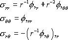
![]()


![]()
We guess that the asymptotic field near the crack tip can be derived from an Airy function that has a separable form
![]()
![]()
![]()
![]()
![]()
where the power ![]()
![]()
![]()
![]()
![]() and
and
![]()
![]()
![]()
![]()
![]() are
to be determined.
are
to be determined.
The strength of the singularity ![]()
![]()
![]()
![]()
![]() can
be determined using the J integral. Evaluating the integral around a
circular contour radius r enclosing the crack tip we obtain
can
be determined using the J integral. Evaluating the integral around a
circular contour radius r enclosing the crack tip we obtain
![]()
![]()
![]()
![]()
![]()
For the J integral to be path independent, it
must be independent of r and therefore W must be of order ![]()
![]()
![]()
![]()
![]() .
The Airy function gives stresses of order
.
The Airy function gives stresses of order ![]()
![]()
![]()
![]()
![]() ,
and the corresponding strain energy density would have order
,
and the corresponding strain energy density would have order ![]()
![]()
![]()
![]()
![]() .
Consequently, for a path independent J, we must have
.
Consequently, for a path independent J, we must have ![]()
![]()
![]()
![]()
![]() , so
, so
![]()
![]()
![]()
![]()
![]()
Note for a linear material (n=1), we recover ![]()
![]()
![]()
![]()
![]() as
expected.
as
expected.
Dimensional considerations therefore indicate that in mode I loading, the stress strain and displacement fields will have the following scaling
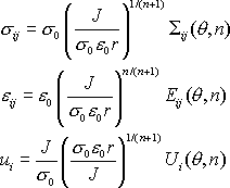


![]()
where ![]()
![]()
![]()
![]()
![]() are
dimensionless functions of the angle
are
dimensionless functions of the angle ![]()
![]()
![]()
![]()
![]() and
the hardening index n only, and J is the value of the J
integral.
and
the hardening index n only, and J is the value of the J
integral.
Note that J plays the role of stress intensity factor in controlling the magnitude of stress, strain and displacement fields at the crack tip. In plastic fracture mechanics, J is used as the fracture criterion instead of K.
To compute ![]()
![]()
![]()
![]()
![]() is
a tedious and not especially straightforward exercise. The governing equation
for the unknown function
is
a tedious and not especially straightforward exercise. The governing equation
for the unknown function ![]()
![]()
![]()
![]()
![]() in
the Airy function is obtained from the condition that the strain field must be
compatible. This requires
in
the Airy function is obtained from the condition that the strain field must be
compatible. This requires
![]()
![]()
![]()
![]()
![]()
Computing the stresses from the Airy function, deducing the strains using the constitutive law and substituting the results into this equation yields a fourth order nonlinear ODE for f, which must be solved subject to appropriate symmetry and boundary conditions. The solution is given in detail in Hutchinson JMPS 16 13 (1968) and Rice and Rosengren ibid, 31.
Phenomenological plastic fracture mechanics based on J
There are many situations (e.g. in design of pressure vessels, pipelines, etc) where the structure is purposely made from a tough, ductile material. Usually, one cannot apply LEFM to these structures, because the a large plastic zone forms at the crack tip (the plastic zone is comparable to specimen dimensions, and there is no K dominant zone). Some other approach is needed to design against fracture in these applications.
Two related approaches are used one based on the HRR crack tip fields and the other based on crack tip opening displacements.
The most important conclusion from the HRR crack tip field is that the amplitude of stresses, strains and displacements near a crack tip in a plastically deforming solid scale in a predictable way with J. Just as stress intensity factors quantify the stress and strain magnitudes in a linear elastic solid, J can be used as a parameter to quantify the state of stress in a plastic solid.
Phenomenological J based fracture mechanics is based on the same reasoning that is used to justify K based LEFM. We postulate that we will observe three distinct regions in a plastically deforming specimen containing a crack,
1. A process zone near the crack tip, with finite deformations and extensive material damge, where the asymptotic HRR field is not accurate
2. A J dominant zone, outside the process zone, but small compared with specimen dimensions, where the HRR field accurately describes the deformation
3. The remainder, where stress and strain fields are controlled by specimen geometry and loading.
As for LEFM, we hope that the process zone is controlled by the surrounding J dominant zone, so that crack tip loading conditions can be characterized by J.
J based fracture mechanics is applied in much the
same way as LEFM. We assume that crack growth starts when J
reaches a critical value (for mode I plane strain loading this value is denoted
![]()
![]()
![]()
![]()
![]() ).
The critical value must be measured experimentally for a given material, using
standard test specimens. To assess the safety of a structure or component
containing a crack, one must calculate J and compare the predicted value
to
).
The critical value must be measured experimentally for a given material, using
standard test specimens. To assess the safety of a structure or component
containing a crack, one must calculate J and compare the predicted value
to ![]()
![]()
![]()
![]()
![]() -
if
-
if ![]()
![]()
![]()
![]()
![]() the
structure is safe.
the
structure is safe.
Practical application of J based fracture
mechanics is somewhat more involved than LEFM. Tests to measure ![]()
![]()
![]()
![]()
![]() are
performed using standard test specimens deeply cracked 3 or 4 point bend bars
are often used. Calibrations for the latter case are available in Rice et
al ASTM STP 536 231 (1973).
are
performed using standard test specimens deeply cracked 3 or 4 point bend bars
are often used. Calibrations for the latter case are available in Rice et
al ASTM STP 536 231 (1973).
Calculating J for a specimen or component
usually requires a full field FEM analysis. Cataloging solutions to
standard problems is much more difficult than for LEFM, because the results
depend on the stress-strain behavior of the material. Specifically, for a
power-law solid containing a crack of length a and subjected to stress ![]()
![]()
![]()
![]()
![]() , we
expect that
, we
expect that
![]()
![]()
![]()
![]()
![]()
For example, a slit crack of length 2a
subjected to mode I loading with stress ![]()
![]()
![]()
![]()
![]() has
(approximately see He & Hutchinson J. Appl. Mech 48 830
1981)
has
(approximately see He & Hutchinson J. Appl. Mech 48 830
1981)
![]()
![]()
![]()
![]()
Finally, to apply the theory it is necessary to
ensure that both test specimen and component satisfy conditions necessary for J
dominance. As a rough rule of thumb, if all characteristic specimen
dimensions (crack length, etc) exceed ![]()
![]()
![]()
![]()
![]() J
dominance is likely to be satisfied.
J
dominance is likely to be satisfied.
Interface cracks
Many engineering applications require one material to be bonded to another. Examples include adhesive joints; protective coatings; composite materials; and thin films used in the manufacture of microelectronic circuits. In all these applications, techniques are required to predict the strength of the bond.
To this end, a great deal of work has been done over the past 20 years to extend linear elastic fracture mechanics to predict the behavior of cracks on, or near, the interface between two dissimilar brittle materials.
Crack Tip Fields for a crack on an interface
As always, the foundation for linear elastic interfacial fracture mechanics is based on an asymptotic analysis of the stress and strain fields near the tip of a crack.
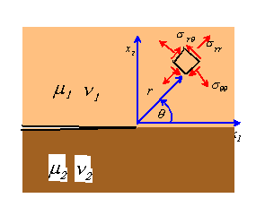
To this end, we consider a semi-infinite crack with
a straight front that coincides with the ![]()
![]()
![]()
![]()
![]() axis,
which lies on the interface between two linear elastic solid, as shown in the
picture. The solid is subjected to static remote loading, and is assumed
to deform in plane strain. We seek a solution to the governing equations
of linear elasto-statics, subject to boundary conditions
axis,
which lies on the interface between two linear elastic solid, as shown in the
picture. The solid is subjected to static remote loading, and is assumed
to deform in plane strain. We seek a solution to the governing equations
of linear elasto-statics, subject to boundary conditions ![]()
![]()
![]()
![]()
![]() on
on
![]()
![]()
![]()
![]()
![]() .
.
The solution will be a function of the elastic
properties of the two bonded materials. For a homogeneous material, the
stress and strain fields for a plane traction boundary value problem are
independent of elastic constants one might therefore expect that for a
bi-material interface problem, the stress and strain fields would depend on two
dimensionless combinations of the four material parameters ![]()
![]()
![]()
![]()
![]() .
This turns out to be the case. Specifically, for a plane problem the
solution can always be expressed in terms of two constants (known as Dundurs
parameters, after their inventor)
.
This turns out to be the case. Specifically, for a plane problem the
solution can always be expressed in terms of two constants (known as Dundurs
parameters, after their inventor)
![]()
![]()
![]()
![]()
![]()
where ![]()
![]()
![]()
![]()
![]() are
the plane strain moduli of the two bonded materials.
are
the plane strain moduli of the two bonded materials.
Evidently ![]()
![]()
![]()
![]()
![]() is
a measure of the relative stiffness of the two materials. It must lie in
the range
is
a measure of the relative stiffness of the two materials. It must lie in
the range ![]()
![]()
![]()
![]()
![]() for
all possible material combinations, with
for
all possible material combinations, with ![]()
![]()
![]()
![]()
![]() signifying
that material 1 is rigid, while
signifying
that material 1 is rigid, while ![]()
![]()
![]()
![]()
![]() signifies
that material 2 is rigid. The second parameter does not have such a nice
physical interpretation it is evidently a measure of the relative
compressibilities of the two materials. For poissons ratios in the range
signifies
that material 2 is rigid. The second parameter does not have such a nice
physical interpretation it is evidently a measure of the relative
compressibilities of the two materials. For poissons ratios in the range
![]()
![]()
![]()
![]()
![]() , we
find that
, we
find that ![]()
![]()
![]()
![]()
![]() .
.
An additional material mismatch parameter appears in interface crack problems, defined by
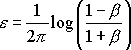
![]()
![]()
![]()
![]()
For most material combinations the value of ![]()
![]()
![]()
![]()
![]() is
very small typically of order 0.01 or so.
is
very small typically of order 0.01 or so.
Asymptotic analysis shows that the crack tip fields for an interface crack may be expressed in the form
![]()
![]()
![]()
![]()
![]()
where ![]()
![]()
![]()
![]()
![]() and
and
![]()
![]()
![]()
![]()
![]() characterize
the remote loading in the same way as mode I and mode II stress intensity
factors for a crack in a homogeneous solid, and
characterize
the remote loading in the same way as mode I and mode II stress intensity
factors for a crack in a homogeneous solid, and ![]()
![]()
![]()
![]()
![]() is
a complex (i.e. it has real and imaginary parts, its not just complicated!)
function of angle and the material mismatch parameter
is
a complex (i.e. it has real and imaginary parts, its not just complicated!)
function of angle and the material mismatch parameter ![]()
![]()
![]()
![]()
![]() .
The function is too complex (i.e. its complicated, in addition to having
real and imaginary parts) to reproduce in full here, but the stress field along
.
The function is too complex (i.e. its complicated, in addition to having
real and imaginary parts) to reproduce in full here, but the stress field along
![]()
![]()
![]()
![]()
![]() has
a simple form
has
a simple form
![]()
![]()
![]()
![]()
![]()
The complex exponent here is scary, but note that
![]()
![]()
![]()
![]()
![]()
so this term indicates that the stresses oscillate near the crack tip. We will discuss this in more detail shortly.
The crack opening displacements have the form
![]()
![]()
![]()
![]()
![]()
where ![]()
![]()
![]()
![]()
![]() is
a plane strain bi-material modulus defined by
is
a plane strain bi-material modulus defined by
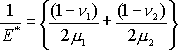
![]()
![]()
![]()
![]()
The energy release rate for the crack is
![]()
![]()
![]()
![]()
![]()
Stress intensity factors for some interface cracks
For a particular crack problem, the stress magnitude (in the K dominant zone) is determined by the complex stress intensity factor
![]()
![]()
![]()
![]()
![]()
The value of K is determined by specimen geometry and loading conditions, exactly as for mode I and mode II stress intensities in homogeneous materials. K has been computed for many standard specimen geometries (usually using a numerical technique). A few examples are shown below.
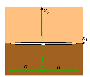
![]()
![]()
![]()
![]()
![]()
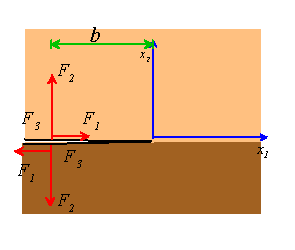
![]()
![]()
![]()
![]()
![]()

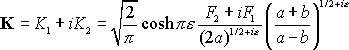
![]()
![]()
![]()
![]()
Note that in all cases the crack tip stress
intensity factors have the functional form ![]()
![]()
![]()
![]()
![]() ,
where Lis a characteristic length.
,
where Lis a characteristic length.
Interpreting the asymptotic field
The asymptotic crack tip field for an interface crack is strikingly different to the corresponding solution for a homogeneous solid. In fact, the results are somewhat disturbing, and have been the cause of much wailing and gnashing of teeth in the fracture mechanics community.
We have already noted that the stress fields are oscillatory near the crack tip. The stress distributions are plotted below as a function of log(r):
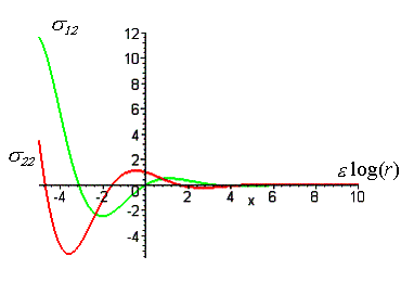
Both normal and shear stresses oscillate with increasing frequency as the crack tip is approached. As a result, it is difficult to unambiguously separate the loading into normal and shear components an opening stress induces just as much shear near the crack tip as does shear loading, and vice-versa.
Even more disturbingly, the crack opening displacements show the same oscillatory character. This means that the solution predicts that the crack faces overlap near the crack tip, which is clearly unphysical.
It is possible to find a solution that corrects for the overlapping crack faces the famous Comninou solution (J. Appl Mech. 44, 631 1977) does just this. This solution predicts that the crack faces touch just behind the crack tip for all combinations of remote load. There is a square root singularity in shear stress at the crack tip (so its strictly always loaded in mode II). The zone of contact is extremely small, however typically of the order of a few nanometers for most practical crack sizes and materials, and probably much smaller than the process zone.
The standard procedure in LEIFM (linear elastic interfacial fracture mechanics) is to ignore the overlap between crack faces, and accept the asymptotic field described in the beginning of this sub-section as characterizing the stress and strain fields for an interface crack. The oscillatory singularity is, after all, no less physical than a square root singularity. The asymptotic field is expected to represent actual stress and strain fields in an annular region, which is small compared with specimen geometry, and large compared with the process zone at the crack tip.
Phenomenological theory of interface fracture
It has become standard to use the complex stress
intensity factor K to characterize the severity of loading near a crack
tip in a bi-material interface. Rather than use ![]()
![]()
![]()
![]()
![]() and
and
![]()
![]()
![]()
![]()
![]() ,
however, the crack tip loading is usually characterized by two parameters
,
however, the crack tip loading is usually characterized by two parameters
1. The energy release rate
![]()
![]()
![]()
![]()
![]()
2. The `phase angle of loading (parameterizing mode mixity), defined as
![]()
![]()
![]()
![]()
![]()
The energy release rate can be computed unambiguously for a given specimen geometry and material pair. This is not the case for the phase angle. Recall that in general
![]()
![]()
![]()
![]()
![]()
so that the ratio ![]()
![]()
![]()
![]()
![]() depends
on a characteristic length and in fact depends on the units used. In
most practical situations this does not lead to serious difficulties, because
the phase angle is such a weak function of
depends
on a characteristic length and in fact depends on the units used. In
most practical situations this does not lead to serious difficulties, because
the phase angle is such a weak function of ![]()
![]()
![]()
![]()
![]() -
since
-
since ![]()
![]()
![]()
![]()
![]() varies
as
varies
as ![]()
![]()
![]()
![]()
![]() and
and
![]()
![]()
![]()
![]()
![]() ,
even an order of magnitude change in L produces an imperceptible change
in phase angle. However, it is important to be aware of this difficulty, and
when reporting experimental measurements of interface toughness, it is
important to specify the characteristic length used in defining the phase
angle.
,
even an order of magnitude change in L produces an imperceptible change
in phase angle. However, it is important to be aware of this difficulty, and
when reporting experimental measurements of interface toughness, it is
important to specify the characteristic length used in defining the phase
angle.
A
![]()
![]()
![]()
![]()
![]()
at the onset of fracture.
Note that the fracture resistance of the interface ![]()
![]()
![]()
![]()
![]() is
a strong function of phase angle
is
a strong function of phase angle ![]()
![]()
![]()
![]()
![]() .
Experimental measurements suggest that
.
Experimental measurements suggest that ![]()
![]()
![]()
![]()
![]() increases
rapidly with phase angle in fact many experimental data seem to be fit by
increases
rapidly with phase angle in fact many experimental data seem to be fit by
![]()
![]()
![]()
![]()
![]()
To apply LEIFM, then, it is necessary (i) to measure the fracture resistance of the interface as a function of phase angle; (ii) calculate energy release rate and phase angle for the interface crack in the structure or component of interest, and (iii) apply the fracture criterion to assess the load bearing capacity of the component.
Several standard specimens are available to measure interfacial fracture toughness. Examples include sandwich specimens (e.g. Leichti & Knauss, Exp. Mech. 22 383 1982; see also Suo & Hutchinson Mat. Sci & Eng A107 1989 135) and 4 point bend specimens (e.g. Charalambides et al Mechanics of Materials 8 269, 1990)
Crack Path Selection
A final issue that is of great interest in interfacial fracture is the question of crack path selection. An interface crack can either propagate along the interface, or deflect into one of the two materials adjacent to the interface. In addition, a crack approaching transverse to an interface may be deflected along it this is a mechanism for trapping cracks in composite materials.
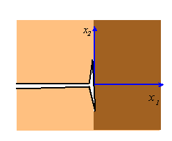
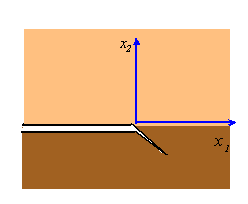
A rather involved stress analysis is requied to answer these questions, but the results are simple. A crack approaching perpendicular to an interface (as shown on the left above) will deflect along the interface as long as
![]()
![]()
![]()
![]()
![]()
where ![]()
![]()
![]()
![]()
![]() is
the interface toughness for a phase angle of 90 degrees, and
is
the interface toughness for a phase angle of 90 degrees, and ![]()
![]()
![]()
![]()
![]() is
the fracture toughness of the material on the far side of the interface.
If this condition is satisfied, the crack remains trapped in the interface and
will not kink out of it.
is
the fracture toughness of the material on the far side of the interface.
If this condition is satisfied, the crack remains trapped in the interface and
will not kink out of it.
|
Politica de confidentialitate | Termeni si conditii de utilizare |

Vizualizari: 1617
Importanta: ![]()
Termeni si conditii de utilizare | Contact
© SCRIGROUP 2024 . All rights reserved