| CATEGORII DOCUMENTE |
| Bulgara | Ceha slovaca | Croata | Engleza | Estona | Finlandeza | Franceza |
| Germana | Italiana | Letona | Lituaniana | Maghiara | Olandeza | Poloneza |
| Sarba | Slovena | Spaniola | Suedeza | Turca | Ucraineana |
1.1. Introduction
If we arrange two electrically isolated coils in such a way that the time-varying flux due to one of them causes an electromotive force (emf) to be induced in the other, they are said to form a transformer.
In other words, a transformer is a device that involves magnetically coupled coils. If only a fraction of the flux produced by one coil links the other, the coils are said to be loosely coupled. In this case, the operation of the transformer is not very efficient.
In order to increase the coupling between the coils, the coils are wound on a common core. When the core is made of a nonmagnetic material, the transformer is called an air-core transformer.
When the core is made of a ferromagnetic material with relatively high permeability, the transformer is referred to as an iron-core transformer.
A highly permeable magnetic core ensures that (a) almost all the flux created by one coil links the other and (b) the reluctance of the magnetic path is low. This results in the most efficient operation of a transformer.
In its simplest form, a transformer consists of two coils that are electrically isolated from each but are wound on the same magnetic core.
A time-varying current in one coil sets up a time-varying flux in the magnetic core. Owing to the high permeability of the core, most of the flux links the other coil and induces a time-varying emf (voltage) in that coil.
The frequency of the induced emf in the other coil is the same as that of the current in the first coil. If the other coil is connected to a load, the induced emf in the coil establishes a current in it. Thus, the power is transferred from one coil to the other via the magnetic flux in the core.
The coil to which the source supplies the power is called the primary winding. The coil that delivers power to the load is called the secondary winding. Either winding may be connected to the source and/or the load.
Since the induced emf in a coil is proportional to the number of turns in a coil, it is possible to have a higher voltage across the secondary than the applied voltage to the primary. In this case, the transformer is called a step-up transformer. A step-up transformer is used to connect a relatively high-voltage transmission line to a relatively low-voltage generator. On the other hand, a step-up transformer has a lower voltage on the secondary side. An example of a step-down transformer is a welding transformer, the secondary of which is designed to deliver a high load current.
When the applied voltage to the primary is equal to the induced emf in the secondary, the transformer is said to have a one-to-one ratio.
A one-to-one ratio transformer is used basically for the purpose of electrically isolating the secondary side from its primary side. Such a transformer is usually called an isolation transformer. An isolation transformer can be utilized for direct current (dc) isolation. That is, if the input voltage on the primary side consists of both dc and alternating current (ac) components, the voltage on the secondary side will be purely ac in nature.
2. 2. Construction of a Transformer
In order to keep the core loss to a minimum, the core of a transformer is built up of thin laminations of highly permeable ferromagnetic material such as silicon-sheet steel. Silicon steel is used because of its nonaging properties and low magnetic losses. The laminations thickness varies from 0.014 inch to 0.024 inch. A thin coating of varnish is applied to both sides of the lamination in order to provide high interlamination resistance. The process of cutting the laminations to the proper size results in punching and shearing strains. These strains cause an increase in the core loss. In order to remove the punching and shearing strains, the laminations are subjected to high temperatures in a controlled environment for some time. It is known as the annealing process.
Basically two types of construction are in common use for the transformers: shell type and core type. In the construction of a shell-type transformer, the two windings are usually wound over the same leg of the magnetic core, as shown in Figure 1.1.
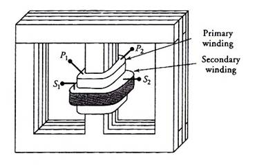
Figure 1.1 Shell-type transformer.
In a core-type transformer, shown in Figure 1.2, each winding may be evenly split and wound on both legs of the rectangular core. The nomenclature, shell type and core type, is derive from the fact that in a shell-type transformer the core encircles the windings, whereas the windings envelop the core in a core-type transformer.
For relatively low power applications with moderate voltage ratings, the windings may be wound directly on the core of the transformer. However, for high-voltage and/or high-power transformers, the coils are usually form-wound and then assembled over the core.
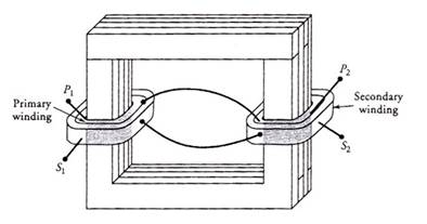
Figure 2.2 Core-type transformer.
Both the core loss (hysteresis and eddy-current loss) and the copper loss (electrical loss) in a transformer generate heat, which, in turn, increases the operating temperature of the transformer. For low-power applications, natural air circulation may be enough to keep the temperature of the transformer within an acceptable range. If the temperature increase cannot be controlled by natural air circulation, a transformer may be cooled by continuously forcing air through its core and windings. When forced-air circulation is not enough, a transformer may be immersed in a transformer oil, which carriers the heat to the walls of the containing tank.
In order to increase the radiating surface of the tank, cooling fins may be welded to the tank or the tank may be built from corrugated sheet steel. These are some of the methods used to curb excessive temperature in the transformer.
3. 3 An Ideal Transformer
A two-winding transformer with each winding acting as a part of a separate electric circuit is shown in Figure 3. 3.
Let N1 and N2 be the number of turns in the primary and secondary windings. The primary winding is connected to a time-varying voltage source v1, while the secondary winding is left open. For the sake of understanding, let us first consider an idealized transformer in which there are no losses and no leakage flux. In other words, we are postulating the following:
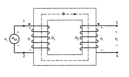
Figure 3.3 An idealized transformer under no load.
According to Faradays law of induction, the magnetic flux F in the core induces an emf e1 in the primary winding that opposes the applied voltage v1.
For the polarities of the applied voltage and the induced emf, as indicated in the figure for the primary winding, we can write
 (1.1)
(1.1)
Similarly, the induced emf in the secondary winding is
 (1.2)
(1.2)
with its polarity as indicated in the figure.
In the idealized case assumed, the induced emfs e1 and e2 are equal to the corresponding terminal voltages v1 and v2, respectively. Thus, from Eqs. (1.1) and (1.2), we obtain
 (1.3)
(1.3)
which states that the ratio of primary to secondary induced emfs is equal to the ratio of primary to secondary turns.
It is a common practice to define the ratio of primary to secondary turns as the a-ratio, or the transformation ratio. That is,
 (1.4)
(1.4)
Let i2 be the current through the secondary winding when it is connected to a load, as shown in Figure 1.4. The magnitude of i2 depends upon the load impedance.
However, its direction is such that it tends to weaken the core flux F and to decrease the induced emf in the primary e1.
For an idealized transformer, e1 must always be equal to v1. In other words, the flux in the core must always be equal to its original no-load value.
In order to restore the flux in the core to its original no-load value, the source v1 forces a current i1 in the primary winding, as indicated in the figure.
In accordance with our assumptions, the mmf of the primary current N1i1 must be equal and opposite to the mmf of the secondary N2i2.
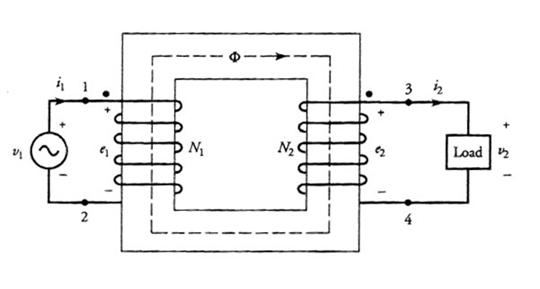
Figure 1. 4 An idealized transformer under load.
In accordance with our assumptions, the mmf of the primary current N1i1 must be equal and opposite to the mmf of the secondary N2i2.
That is,
![]()
or
 (1.5)
(1.5)
which states that the primary and the secondary currents are transformed in the inverse ratio of turns.
![]() (1.6)
(1.6)
This equation simply confirms our assumption of no losses in an idealized transformer. It highlights the fact that, at any instant, the power output (delivered to the load) is equal to the power input (supplied by the source).
For sinusoidal variations in the applied voltage, the magnetic flux in the core also varies sinusoidally under ideal conditions. If the flux in the core at any instant t is given as
![]()
where Fm is the
amplitude of the flux and ![]() is the angular frequency, then the induced emf in the primary
is
is the angular frequency, then the induced emf in the primary
is
![]()
The above equation can be expressed in phasor form in terms of its root-mean-square (rms) or effective value as
![]()
 (1.7)
(1.7)
![]()
Likewise, the induced emf in the secondary winding is
![]() (1.8)
(1.8)
From Eqs. (1.7) and (1.8), we get
 (1.9)
(1.9)
where ![]() and
and ![]() under ideal
conditions. From the above equation, it is obvious that the induced emfs are in
phase. For an idealized transformer, the terminal voltages are also in phase.
under ideal
conditions. From the above equation, it is obvious that the induced emfs are in
phase. For an idealized transformer, the terminal voltages are also in phase.
 (1.10)
where ![]() and
and ![]() are the currents in
phasor form through the primary and secondary windings. The above equation
dictates that and must be in phase for an idealized transformer.
are the currents in
phasor form through the primary and secondary windings. The above equation
dictates that and must be in phase for an idealized transformer.
Equation (4.6) can also be expressed in terms of phasor quantities as
![]() (1.11)
(1.11)
That is, the complex power supplied to the primary winding by the source is equal to the complex power delivered to the load by the secondary winding, in terms of the apparent powers, the above equation becomes
![]() (1.12)
(1.12)
or
![]() (1.13)
(1.13)
where ![]() is the load impedance
as referred to the primary side. Equation (4.13) states that the load
impedance as seen by the source on the primary side is equal to a2
times the actual load impedance on the secondary side.
is the load impedance
as referred to the primary side. Equation (4.13) states that the load
impedance as seen by the source on the primary side is equal to a2
times the actual load impedance on the secondary side.
This equations states that a transformer can also be used for impedance matching. A known impedance can be raised or lowered to match the rest of the circuit for maximum power transfer.
A transformer may have multiple windings that may be connected either in series to increase the voltage rating or in parallel to increase the current rating. Before the connections are made, however, it is necessary that we know the polarity of each winding. By polarity we mean the relative direction of the induced emf in each winding.
Let us examine the transformer shown in Figure 1.4.
Let the polarity of the time-varying source connected to the primary winding, at any instant, be as indicated in the figure.
Since the induced emf e1 in the primary of an idealized transformer must be equal and opposite to the applied voltage v1, terminal 1 of the primary is positive with respect to terminal 2.
The wound direction of primary winding as shown in the figure is responsible for the clockwise direction of the flux F in the core of the transformer. This flux must induce in the secondary winding an emf e2 that results in the current i2 as indicated. The direction of the current i2 is such that it produces a flux that opposes the change in the original flux F. For the wound direction of the secondary winding as depicted in the figure, terminal 3 must be positive with respect to terminal 4. Since terminal 3 has the same polarity as terminal 1, they are said to follow each other. In other words, terminals 1 and 3 are like-polarity terminals. To indicate the like-polarity relation-ship, we have placed dots at these terminals.
The nameplate of a transformer provides information on the apparent power and the voltage-handling capacity of each winding. From the nameplate data of a 5-kVA, 500/250-V, step-down transformer, we conclude the following:
![]()
and
![]()
Since the information on the number of turns is customarily not given by manufacturer, we determine the a-ratio from the (nominal) terminal volt as
 .
.
1.4. A Nonideal Transformer
In the previous section we placed quite a few restrictions to obtain useful relations for an idealized transformer. In this section, our aim is to lift those restrictions in order to develop an equivalent circuit for a nonideal transformer.
Winding Resistances
However small it may be, each winding has some resistance. Nonetheless, we can replace a nonideal transformer with an idealized transformer by including a lumped resistance equal to the winding resistance of series with each winding. As shown in Figure 1.6, R1 and R2 are the winding resistances of the primary and the secondary, respectively.
The inclusion of the winding resistances dictates that (a) the power input must be greater than the power output, (b) the terminal voltage is not equal to the induced emf, and (c) the efficiency (the ratio of power out-put to power input) of a nonideal transformer is less than 100%.
Not all of the flux created by a winding confines itself to the magnetic core on which the winding is wound. Part of the flux, known as the leakage flux, does complete its path through air. Therefore, when both windings in a transformer carry currents, each creates its own leakage flux, as illustrated in Figure 1.7. The primary leakage flux set up by the primary does not link the secondary. Likewise, the secondary leakage flux restricts itself to the secondary and does not link the primary. The common flux that circulates in the core and links both windings is termed the mutual flux.
Although a leakage flux is a small fraction of the total flux created by a winding, it does affect the performance of a transformer. We can model a winding as if it consists of two windings: One winding is responsible to create the leakage flux through air, and the other encircles the core. Such hypothetical winding arrangements are shown in Figure 1.8 for a two-winding transformer.
The two windings enveloping the core now satisfy the conditions of an idealized transformer.
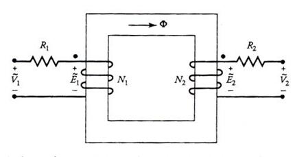
Figure 1.6 An ideal transformer with winding resistances modelled as lumped resistances.
The leakage flux associated with either winding is responsible for the voltage drop across it. Therefore, we can represent the voltage drop due to the leakage flux by a leakage reactance, as discussed in Chapter 2. If X1 and X2 are the leakage reactances of the primary and secondary windings, a real transformer can then be represented in terms of an idealized transformer with winding resistance and leakage reactances as shown in Figure 1.9.
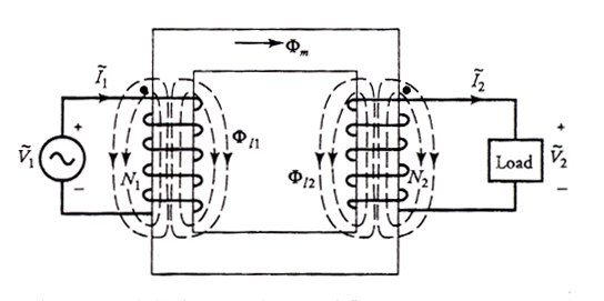
Figure 1.7 Transformer with leakage and mutual fluxes.
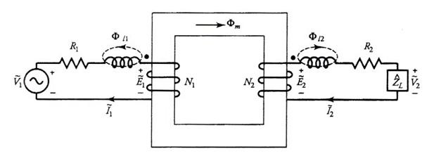
Figure 1. 8 Hypothetical windings showing leakage and mutual flux linkages separately.
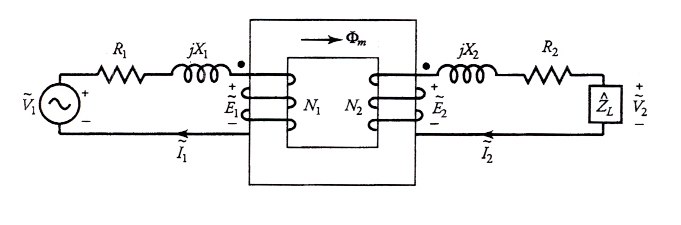
Figure 1.9 A nonideal transformer represented in terms of an ideal transformer with winding resistances and leakage reactances.
In the case of a nonideal transformer

![]()
and
![]()
Note that in a
nonideal transformer, ![]() and
and ![]() .
.
Finite Permeability
The core of a
nonideal transformer has finite
permeability and core loss. Therefore, even when the secondary is left open
(no-load condition) the primary winding draws some current, known as the excitation current, from the source. It
is a common practice to assume that the excitation current, ![]() , is the sum of two currents, the core-loss current,
, is the sum of two currents, the core-loss current, ![]() , and the magnetizing
current,
, and the magnetizing
current, ![]() .
.
That is,
![]() (1.14)
(1.14)
The
core-loss component of the excitation current accounts for the magnetic loss (the hysteresis loss and the
eddy-current loss) in the core of a transformer. If ![]() is the induced emf on
the primary side and Rc1
is the equivalent core-loss resistance, then the core-loss current,
is the induced emf on
the primary side and Rc1
is the equivalent core-loss resistance, then the core-loss current, ![]() , is
, is
 (1.15)
The
magnetizing component of the excitation current is responsible to set up the
mutual flux in the core. Since a current-carrying coil forms and inductor, the
magnetizing current, ![]() , gives rise to a magnetizing
reactance, Xm1.
Thus,
, gives rise to a magnetizing
reactance, Xm1.
Thus,
 (1.16)
We can now modify the equivalent circuit of Figure 1. 9 to include the core-loss resistance and the magnetizing reactance. Such a circuit is shown in Figure 1.10.
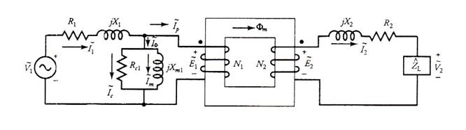
Figure 1.10 Equivalent circuit of a transformer including winding resistances, leakage reactance, core-loss resistance, magnetizing reactance, and an ideal transformer.
We can now modify the equivalent circuit of Figure 1.9 to include the core-loss resistance and the magnetizing reactance. Such a circuit is shown in Figure 1.10.
When we increase the load on the transformer, the following sequence of events takes place:
(a) The secondary winding current increases.
(b) The current supplied by the source increases.
(c)
The voltage drop across the primary
winding impedance ![]() increases
increases
(d)
The induced emf ![]() drops.
drops.
(e) Finally, the mutual flux decreases owing to the decrease in the magnetizing current.
However,
in a well-designed transformer, the decrease in the mutual flux from no load to
full load is about 1% to 3%. Therefore, for all practical purposes, we can
assume that ![]() remains substantially
the same. In other words, the mutual flux is essentially the same under normal
loading conditions and thereby there is no appreciable change in the excitation
current.
remains substantially
the same. In other words, the mutual flux is essentially the same under normal
loading conditions and thereby there is no appreciable change in the excitation
current.
In the equivalent circuit representation of a transformer, the core is rarely shown. Sometimes, parallel lines are drawn between the two windings to indicate the presence of a magnetic core. We will use such an equivalent circuit representation.
If the parallel lines between the two windings are missing, our interpretation is that the core is nonmagnetic. With that understanding, the exact equivalent circuit of a real transformer is given in Figure 1.11.
In this figure,
a dashed box is also drawn to shown that the circuit enclosed by it is the
so-called ideal transformer. All the ideal- transformer relationships can be
applied to this circuit. The load current ![]() on the secondary side
is represented on the primary side as
on the secondary side
is represented on the primary side as ![]() .
.
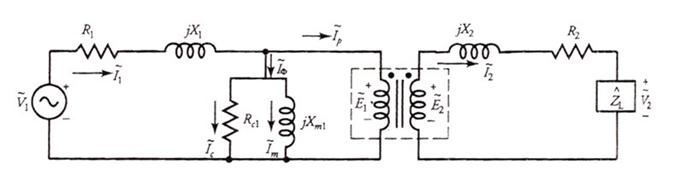
Figure 1.11 An exact equivalent circuit of a real transformer. The coupled-coiled in the dashed box represent an ideal transformer with a magnetic core.
The excitation current can now be determined as
 (1.17)
It is possible to represent a transformer by an equivalent circuit that does not employ an ideal transformer. Such equivalent circuits are drawn with reference to a given winding. Figure 1.12 shows such an equivalent circuit as viewed from the primary side. Note that the circuit elements that were on the secondary side in Figure 1.11 have been transformed to the primary side in Figure 1.12. Figure 1.13 shows the equivalent circuit of the same transformer as referred to the secondary side.
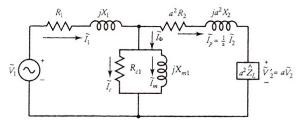
Figure 1.12 The exact equivalent circuit as viewed from the primary side of the transformer.
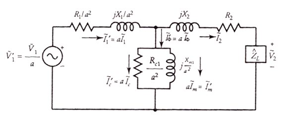
Figure 1.13 An exact equivalent circuit as viewed from the secondary side of the transformer.
Phasor Diagram
When a transformer operates under steady-state conditions, an insight into its currents, voltages, and phase angles can be obtained by sketching its phasor diagram. Even though a phasor diagram can be developed by using any phasor quantity as a reference, we use the load voltage as a reference because quite often it is a known quantity.
Let
![]() be the voltage across
the load impedance
be the voltage across
the load impedance ![]() and
and ![]() be the load current.
Depending upon
be the load current.
Depending upon ![]() ,
, ![]() may be leading, in
phase with, or lagging
may be leading, in
phase with, or lagging ![]() . In this particular case, let us assume that
. In this particular case, let us assume that ![]() lags
lags ![]() by an angle q2.
We first draw a horizontal line from the origin of magnitude V2 to represent the phasor
by an angle q2.
We first draw a horizontal line from the origin of magnitude V2 to represent the phasor ![]() , as shown in Figure 1.14. The current I2 is now drawn lagging V2 by q2.
, as shown in Figure 1.14. The current I2 is now drawn lagging V2 by q2.
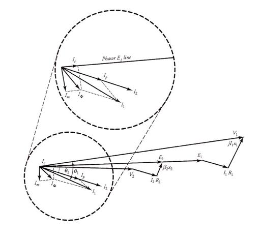
Figure 1.14 The phasor diagram of a nonideal transformer as shown in Figure 1.11.
From the equivalent circuit, Figure 1.11, we have
![]()
We now proceed
to construct the phasor diagram for E2. Since the voltage
drop ![]() is in phase with
is in phase with ![]() and it is to be added
to
and it is to be added
to ![]() , we draw a line of magnitude I2R2 starting at the tip of
V2
and parallel to I2. The length of the line from the origin to the
tip of I2R2
represents the sum of
, we draw a line of magnitude I2R2 starting at the tip of
V2
and parallel to I2. The length of the line from the origin to the
tip of I2R2
represents the sum of ![]() and
and ![]() . We can now add the voltage drop
. We can now add the voltage drop ![]() at the tip of I2R2 by drawing a line equal to its magnitude and leading
at the tip of I2R2 by drawing a line equal to its magnitude and leading ![]() by 90o. A
line from the origin to the tip of
by 90o. A
line from the origin to the tip of ![]() represents the
magnitude of
represents the
magnitude of ![]() . This completes the phasor diagram for the secondary
winding.
. This completes the phasor diagram for the secondary
winding.
Since
![]() , the magnitude of the induced emf on the primary side
depends upon the a-ratio. Let us
assume that the a-ratio is greater
than unity. In that case,
, the magnitude of the induced emf on the primary side
depends upon the a-ratio. Let us
assume that the a-ratio is greater
than unity. In that case, ![]() is greater than
is greater than ![]() and can be represented
by extending E2 as shown.
and can be represented
by extending E2 as shown.
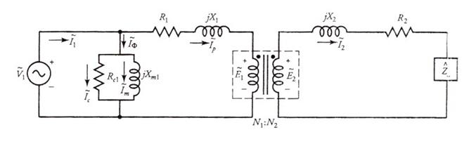
Figure 1.15 An approximate equivalent circuit of a transformer embodying an ideal transformer.
The
current ![]() is in phase with
is in phase with ![]() , and
, and ![]() lags
lags ![]() by 90o.
These currents are draw from the origin as shown. The sum of these currents
yields the excitation current
by 90o.
These currents are draw from the origin as shown. The sum of these currents
yields the excitation current ![]() . The source current I1
is now constructed using the currents If
and I2/a, as illustrated in the figure. The
voltage drop across the primary-winding impedance
. The source current I1
is now constructed using the currents If
and I2/a, as illustrated in the figure. The
voltage drop across the primary-winding impedance ![]() is now added to obtain
the phasor
is now added to obtain
the phasor ![]() . The phasor diagram is now complete. In this case, the
source current
. The phasor diagram is now complete. In this case, the
source current ![]() lags the source
voltage
lags the source
voltage ![]() by an angle q.
by an angle q.
Phasor diagrams for the exact equivalent circuits as shown in Figures 1.12 and 1.13 cal also be drawn and are left as exercises for the reader.
Approximate Equivalent Circuits
In a
well-designed transformer, the winding resistances, the leakage reactances and
the core loss are kept as low as possible. The low core loss implies high
core-loss resistance. The high permeability of the core ensures high
magnetizing reactance. Thus, the impedance of the so-called parallel branch (Rc1 in parallel
with jXm1)
across the primary is very high compared with ![]() and
and ![]() . The high impedance of the parallel branch assures low
excitation current, In the analysis of complex power systems, a great deal of
simplification can be achieved by neglecting the excitation current.
. The high impedance of the parallel branch assures low
excitation current, In the analysis of complex power systems, a great deal of
simplification can be achieved by neglecting the excitation current.
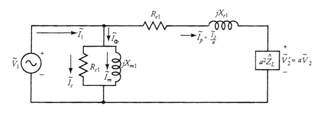
Figure 4.16 Approximate equivalent circuit of a transformer as viewed from the primary side.
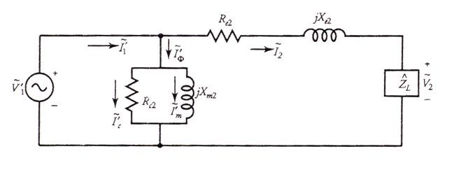
Figure 4.17 An approximate equivalent circuit of a transformer as viewed from the secondary side.
Since
![]() is kept low, the voltage drop across it is also low
in comparison with the applied voltage. Without introducing any appreciable
error in our calculations, we can assume that the voltage drop across the
parallel branch is the same as the applied voltage. This assumption allows us
to move the parallel branch as indicated in Figure 1.15 for the equivalent
circuit of a transformer embodying an ideal transformer. This is referred to as
the approximate equivalent circuit of a
transformer.
is kept low, the voltage drop across it is also low
in comparison with the applied voltage. Without introducing any appreciable
error in our calculations, we can assume that the voltage drop across the
parallel branch is the same as the applied voltage. This assumption allows us
to move the parallel branch as indicated in Figure 1.15 for the equivalent
circuit of a transformer embodying an ideal transformer. This is referred to as
the approximate equivalent circuit of a
transformer.
The approximate equivalent circuit as viewed from the primary side is given in Figure 1.16, where
![]() (1.18a)
(1.18a)
![]() (1.18b)
(1.18b)
and
![]() (1.18c)
(1.18c)
Similarly, Figure 1.17 shows the approximate equivalent circuit as referred to the secondary side of the transformer. In this figure,
![]() (1.19a)
(1.19a)
 (1.19b)
 (1.19c)
 (1.19d)
 . (1.19e)
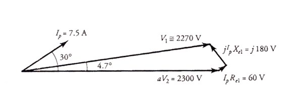
Figure 1.18 The phasor diagram of a transformer discussed in Example 1.5.
1.5. Voltage Regulation
Consider a transformer whose primary winding voltage is adjusted so that it delivers the rated load at the rated secondary terminal voltage. If we now remove the load, the secondary terminal voltage changes because of the change in the voltage drops across the winding resistances and leakage reactances. A quantity of interest is the net change in the secondary winding voltage from no load to full load for the same primary winding voltage. When the change is expressed as a percentage of its rated voltage, it is called the voltage regulation (VR) or the transformer. As a percent, it may be written as
 (1.20)
where V2NL and V2FL are the effective values of no-load and full-load voltages at the secondary terminals.
The voltage regulation is like the figure-of-merit of a transformer. For an ideal transformer, the voltage regulation is zero. The smaller the voltage regulation, the better the operation of the transformer.
1.6 Maximum Efficiency Criterion
As defined earlier, the efficiency is simply the ratio of power output to power input. In a real transformer, the efficiency is always less than 100% owing to the two types of losses: the magnetic loss and the copper loss.
The magnetic loss, which is commonly referred to as the core loss, consists of eddy-current loss and hysteresis loss. For a given flux density and the frequency of operation, the eddy-current loss can be minimized by using thinner laminations. On the other hand, the hysteresis loss depends upon the magnetic characteristics of the type of steel used for the magnetic core. Since the flux, Fm, in the core of a transformer is practically constant for all conditions of load, the core (magnetic) loss, Pm, is essentially constant. It is for this reason that the core loss is often referred to as the fixed loss.
The copper loss (also known as I2R loss or the electric-power loss) comprises the power dissipated by the primary and secondary windings. The copper loss, Pcu varies as the square of the current in each winding. Therefore, as the load increases, so does the copper loss. That is why the copper loss is also termed the variable loss.
The power output can be obtained simply by subtracting the core loss and the copper loss from the power input. This implies that we can also obtain power input by adding the core loss and the copper loss to the power output. We can highlight the power flow from the input toward the output by a single-line diagram, called the power-flow diagram. A power-flow diagram of a transformer (see Figure 1.11) is shown in Figure 1.19.
The efficiency of a transformer is zero at no load. It increases with the increase in the load and rises to a maximum value. Any further increase in the load actually forces the efficiency of a transformer to drop off. Therefore, there exists a definite load for which the efficiency of a transformer is maximum. We now proceed to determine the criterion for the maximum efficiency of a transformer.
Let
us consider the approximate equivalent circuit of a transformer as viewed from
the primary side (see Figure 1.16). The equivalent load current and the load
voltage on the primary side are ![]() and aV2. The power output is
and aV2. The power output is
![]()
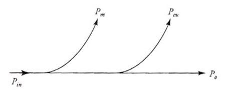
Figure 1.19 Power-flow diagram of a transformer.
And the copper loss is
![]()
If the core loss is Pm, then the power input is
![]()
Hence the efficiency of the transformer is

The only variable in the above equation is the load current Ip for a given load impedance. Therefore, if we differentiate it with respect to Ip and set it equal to zero, we obtain
![]() (1.23a)
(1.23a)
where Iph is the load current on the primary side at maximum efficiency. The above equation states that the efficiency of a transformer is maximum when the copper loss is equal to the core (magnetic) loss. In other words, a transformer operates at its maximum efficiency when the copper-loss curve intersects the core-loss curve, as depicted in Figure 4.20.
We can rewrite Eq. (1.23a) as
 (1.23b)
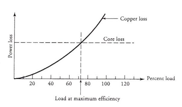
Figure 1.20 Losses in a transformer.
If Ipf1 is the full-load current on the primary side, then the above equation can also be written as
or
 (1.24)
where ![]() is the copper loss at
full load.
is the copper loss at
full load.
Multiplying both sides of Eq. (1.24) by the rated load voltage on the primary side (aV2), we can obtain the rating of the transformer at maximum efficiency in terms of its nominal rating as
 (1.25)
The volt-ampere rating at maximum efficiency can actually be determined by performing tests on the transformer as explained in the ensuing section.
EXEMPLE
A 120-kVA, 2400/240-V, step-down transformer has the following parameters: R1 = 0.75 W, X1 = 0.8 W, R2 = 0.01 W, X2 = 0.02 W. The transformer is designed to operate at maximum efficiency at 70% of its rated load with 0.8 pf lagging. Determine (a) the kVA rating of the transformer at maximum efficiency, (b) the maximum efficiency, (c) the efficiency at full load and 0.8 pf lagging, and (d) the equivalent core-loss resistance.
S O L U T I O N
Let us use approximate equivalent circuit of the transformer as shown in Figure 4.16. The rated voltage across the load as viewed from the primary side is 2400 V. Thus, the rated load current is

The load current at maximum efficiency is
![]()
(a) The kVA rating of the transformer at maximum efficiency is

Thus, the copper loss at maximum efficiency is
![]()
and the core loss is
![]()
(b) The power output, the power input, and the efficiency when the transformer delivers the load at maximum efficiency are
![]()
![]()
![]()
 or 94%
(c) The power output, the copper loss, and the efficiency at full load are
![]()
![]()
 or 93,6%
(d) The equivalent core-loss resistance at no load is

1.7 Determination of Transformer Parameters
The equivalent circuit parameters of a transformer can be determined by performing two tests: the open-circuit test and the short-circuit test.
The Open-Circuit Test
As the name implies, one winding of the transformer is left open while the other is excited by applying the rated voltage. The frequency of the applied voltage must be the rated frequency of the transformer. Although it does not matter which side of the transformer is excited, it is safer to conduct the test on the low-voltage side. Another justification for performing the test on the low-voltage side is the availability of the low-voltage source in any test facility.
Figure 1.21 shows the connection diagram for the open-circuit test with ammeter, voltmeter, and wattmeter inserted on the low-voltage side. If we assume that the power loss under no load in the low-voltage winding is negligible, then the corresponding approximate equivalent circuit as viewed from the low-voltage side is given in Figure 1.22. From the approximate equivalent of the transformer as referred to the low-voltage side (Figure 1.22), it is evident that the source supplies the excitation current under no load. One component of the excitation current is responsible for the core loss, whereas the other is responsible to establish the required flux in the magnetic core. In order to measure these values exactly, the source voltage must be adjusted carefully to its rated value. Since the only power loss in Figure 1.22 is the core loss, the wattmeter measures the core loss in the transformer.
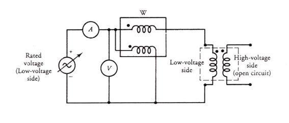
Figure 1.21 A two-winding transformer wired with instruments for open-circuit test.
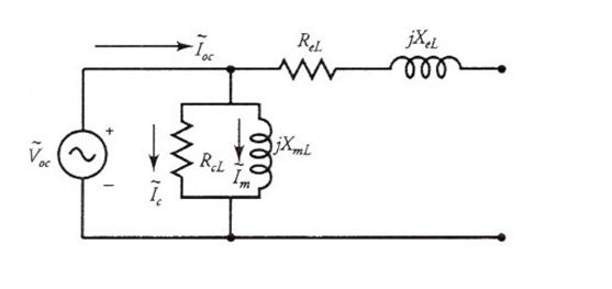
Figure 1.22 The approximate equivalent circuit of a two-winding transformer under open-circuit test.
The core-loss component of the excitation current is in phase with the applied voltage while the magnetizing current lags the applied voltage by 90o, as shown in Figure 4.23. If V0c is the rated voltage applied on the low-voltage side, I0c is the excitation current as measured by the ammeter, and P0c is the power recorded by the wattmeter, then the apparent power at no-load is
![]()
at a lagging power-factor angle of
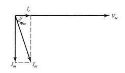
Figure 1.23 The phasor diagram of a two-winding transformer under open-circuit test.
The core-loss and magnetizing currents are
![]()
and
![]()
Thus, the core-loss resistance and the magnetizing reactance as viewed from the low-voltage side are
 (1.26)
and
 (1.27)
where
![]()
The Short-Circuit Test
This test is designed to determine the winding resistances and leakage reactances. The short-circuit test is conducted by placing a short circuit across one winding and exciting the other from an alternating-voltage source of the frequency at which the transformer is rated. The applied voltage is carefully adjusted so that each winding carries a rated current. The rated current in each winding ensures a proper simulation of the leakage flux pattern associated with that winding. Since the short circuit constrains the power output to be zero, the power input to the transformer is low. The low power input at the rated current implies that the applied voltage is a small fraction of the rated voltage. Therefore, extreme care must be exercised in performing this test.
Once again, it does not really matter on which side this test is performed. However, the measurement of the rated current suggests that, for safety purposes, the test be performed on the high-voltage side. The test arrangement with all instruments inserted on the high-voltage side with a short circuit on the low-voltage side is shown in Figure 1.24.
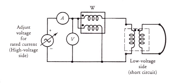
Figure 1.24 A two-winding transformer wired for short-circuit test.
Since the applied voltage is a small fraction of the rated voltage, both the core-loss and the magnetizing currents are so small that they can be neglected. In other words, the core loss is practically zero and the magnetizing reactance is almost infinite. The approximate equivalent circuit of the transformer as viewed from the high-voltage side is given in Figure 1.25. In this case, the wattmeter records the copper loss at full load.
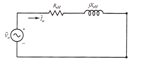
Figure 1.25 An approximate equivalent circuit of a two-winding transformer under short-circuit condition.
If Vsc, Isc, and Psc are the readings on the voltmeter, ammeter, and wattmeter, then
 (1.28)
is the total resistance of the two windings as referred to the high-voltage side.
The magnitude of the impedance as referred to the high-voltage side is
 (1.29)
Therefore, the total leakage reactance of the two windings as referred to the high-voltage side is
![]() (1.30)
(1.30)
If we define the a-ratio as

then
![]() (1.31)
(1.31)
and
![]() (1.32)
(1.32)
where RH is the resistance of the high-voltage winding, RL is the resistance of the low-voltage winding, XH is the leakage reactance of the high-voltage winding, and XL is the leakage reactance of the low-voltage winding.
If the transformer is available, we can measure RH and RL and verify Eq. (1.31). However, there is no simple way to separate the two leakage reactances. The same is also true for the winding resistances if the transformer is unavailable. If we have to segregate the resistances, we will assume that the transformer has been designed in such a way that the power loss on the high-voltage side is equal to the power loss on the low-voltage side. This is called the optimum design criterion and under this criterion
![]()
which yields
![]() (1.33)
(1.33)
Similarly, we can assume that
![]() (1.34)
(1.34)
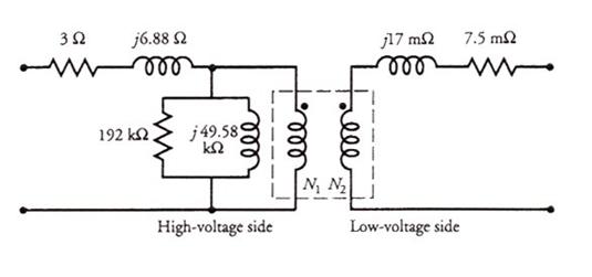
Figure 1.28 The exact equivalent circuit of a transformer for Example 1.8.
The exact equivalent circuit incorporating an ideal transformer is shown in Figure 1.28.
1. 8 Per-Unit Computations
When an electric machine is designed or analyzed using the actual values of its parameters, it is not immediately obvious how its performance compares with another similar-type machine. However, if we express the parameters of a machine as a per-unit (pu) of a base (or reference) value, we will find that the per-unit values of machines of the same type but widely different ratings lie within a narrow range. This is one of the main advantages of a per-unit system.
An electric system has four quantities of interest: voltage, current, apparent power, and impedance. If we select base values of any two of them, the base values of the remaining two can be calculated. If Sb is the apparent base power and Vb is the base voltage, then the base current and base impedance are
 (1.35)
 (1.36)
The actual quantity can now be expressed as a decimal fraction of its base value by using the following equation.
 (1.37)
Since the power rating of a transformer is the same on both sides, we can use it as one of the base quantities. However, we have to select two base voltages - one for the primary side and the other for the secondary side. The two base voltages must be related by the a-ration. That is,
 (1.38)
where VbH and VbL are the base voltages on the high- and low-voltage sides of a transformer, respectively.
Since the base voltages have been transformer, the currents and impedances are also transformed. In other words, the a-ratio is unity when the parameters of a transformer are expressed in terms of their per-unit values. The following example illustrates the analysis of a transformer on a per-unit basis.
1.9 The Autotransformer
In the two-winding transformer we have considered thus far, the primary winding is electrically isolated from the secondary winding. The two windings are coupled together magnetically by a common core. Thus, the principle of magnetic induction is responsible for the energy transfer from the primary to the secondary.
When the two windings of a transformer are interconnected electrically, it is called an autotransformer. An autotransformer may have a single continuous winding that is common to both the primary and the secondary.
Alternatively we can connect two or more distinct coils wound on the same magnetic core to form an autotransformer. The principle of operation is the same in ether case
The direct electrical connection between the windings ensures that a part of the energy is transferred from the primary to the secondary by conduction. The magnetic coupling between the windings guarantees that some of the energy is also delivered by induction.
Autotransformers may be used for almost all applications in which we use a two-winding transformer. The only disadvantage in doing so is the loss of electrical isolation between the high- and low-voltage sides on the autotransformer. Listed below are some of the advantages of an autotransformer compared with a two-winding transformer.
It is cheaper in first cost than a conventional two-winding transformer of a similar rating.
It delivers more power than a two-winding transformer of similar physical dimensions.
For a similar power rating, an autotransformer is more efficient than a two-winding transformer.
An autotransformer requires lower excitation current than a two-winding transformer to establish the same flux in the core.
We begin our discussion of an autotransformer by connecting an ideal two-winding transformer as an autotransformer. In fact, there are four possible ways to connect a two-winding transformer as an autotransformer, as shown in Figure 1.31.
Let us consider the circuit shown in Figure 1.13a.
The two-winding transformer is connected as a step-down autotransformer. Note that the secondary winding of the two-winding transformer is now the common winding for the autotransformer. Under ideal conditions,
![]()
![]()
 (1.39)
where a = N1/N2 is the a-ratio of a two-winding transformer, and aT = 1 + a is the a-ratio of the autotransformer under consideration.
The a-ratio for the other connections should also be computed in the same way. Note that At is not the same for all connections.
In an ideal autotransformer, the primary mmf must be equal and opposite of the secondary mmf. That is,
![]()
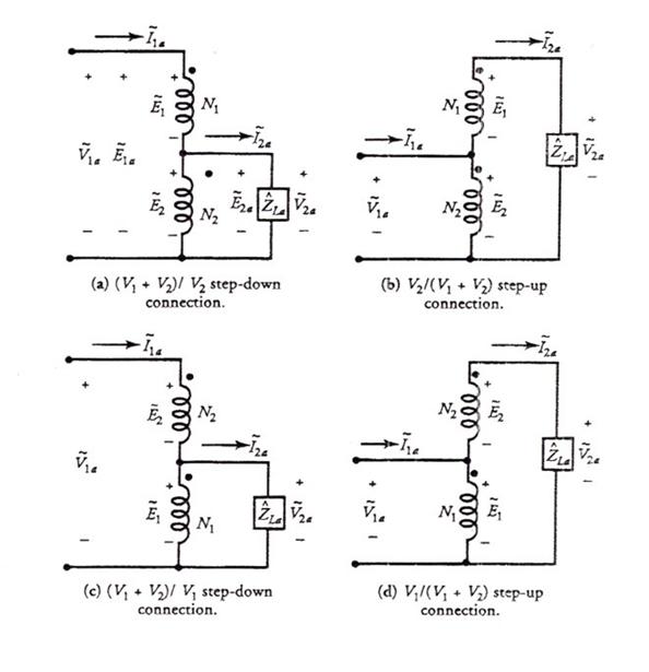 Figure 1.31 Possible ways to connect a
two-winding transformer as an autotransformer.
Figure 1.31 Possible ways to connect a
two-winding transformer as an autotransformer.
From this equation, we obtain
 (1.40)
Thus, the apparent power supplied by an ideal transformer to the load, S0a, is
 (1.41)
where Sina is the apparent input to the autotransformer.
The above equation simply highlights the fact that the power input is equal to the power output under ideal conditions.
Let us now express the apparent output power in terms of the parameters of a two-winding transformer. For the configuration under consideration,
![]()
and
![]()
However, for the rated load, I1a = I1. Thus,
![]()

where S0 = V2I2 is the apparent power output of a two-winding transformer.
This power is associated with the common winding of the autotransformer. This, therefore, is the power transferred to the load by induction in an autotransformer. The rest of the power, S0/a in this case, is conducted directly from the source to the load and is called the conduction power. Hence, a two-winding transformer delivers more power when connected as an autotransformer.
1.10 Three-Phase Transformers
Since most of the power generated and transmitted over long distances is of the three-phase type, we can use three exactly alike single-phase transformers to form a single three-phase transformer. For economic reasons, however, a three-phase transformer is designed to have all six windings on a common magnetic core. A common magnetic core, three-phase transformer can also be either a core type (Figure 1.35) or a shell type (Figure 1.36).
Since the third harmonic flux created by each winding is in phase, a shell-type transformer is preferred because it provides an external path for this flux. In other words, the voltage waveforms are less distorted for a shell-type transformer than for a core-type transformer of similar ratings.
The three windings on either side of a three-phase transformer can be connected either in wye (Y) or in delta (D). Therefore, a three-phase transformer can be connected in four possible ways: Y/Y, Y/D, D/Y, and D/D. Some of the advantages and drawbacks of each connection are highlighted below.
Y/Y Connection
A Y/Y connection
for the primary and secondary windings of a three-phase transformer is depicted
in Figure 1.37. The line-to-line voltage on each side of the three-phase
transformer is ![]() times the nominal
voltage of the single-phase transformer. The main advantage of a Y/Y connection
is that we have access to the neutral terminal on each side and it can be
grounded if desired. Without grounding the neutral terminals, the Y/Y operation
is satisfactory only when the three-phase load is balanced. The electrical
insulation is stressed only to about 58% of the line voltage in a Y-connected
transformer.
times the nominal
voltage of the single-phase transformer. The main advantage of a Y/Y connection
is that we have access to the neutral terminal on each side and it can be
grounded if desired. Without grounding the neutral terminals, the Y/Y operation
is satisfactory only when the three-phase load is balanced. The electrical
insulation is stressed only to about 58% of the line voltage in a Y-connected
transformer.
Since most of the transformers are designed to operate at or above the knee of the curve, such a design causes the induced emfs and currents to be distorted. The reason is as follows: Although the excitation currents are still 120o out of phase with respect to each other, their waveforms are no more sinusoidal. These currents, therefore, do not add up to zero. If the neutral is not grounded, these currents are forced to add up to zero. Thus, they affect the waveforms of the induced emfs.
D/D Connection
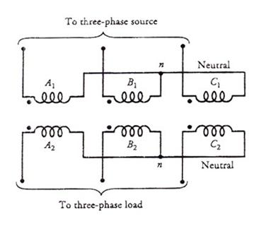
Figure 1.37 A Y/Y-connected three- phase transformer.
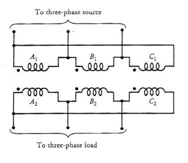
Figure 1.38 A D/D-connected three-phase transformer.
Figure 1.38 shows the three transformers with the primary and secondary windings connected as D/D. The line-to-line voltage on either side is equal to the corresponding phase voltage. Therefore, this arrangement is useful when the voltages are not very high. The advantage of this connection is that even under unbalanced loads the three-phase load voltages remain substantially equal. The disadvantage of the D/D-connection is the absence of a neutral terminal on either side. Another drawback is that the electrical insulation is stressed to the line voltage. Therefore, a D-connected winding requires more expensive insulation that a Y-connected winding for the same power rating.
A D/D-connection can be analyzed theoretically by transforming it into a simulated Y/Y connection using D-to-Y transformations.
Y/D Connection
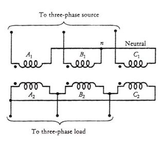
Figure 1.39 A Y/D-connected three-phase transformer.
This connection, as shown in Figure 1.39, is very suitable for step-down applications. The secondary winding current is about 58% of the load current. On the primary side the voltages are form line to neutral, whereas the voltages are from line to line on the secondary side.
Therefore, the voltage and the current in the primary are out of phase the voltage and the current in the secondary. In a Y/D connection, the distortion in the waveform of the induced voltages is not as drastic as it is in a Y/Y- connected transformer when the neutral is not connected to the ground. The reason is that the distorted currents in the primary give rise to a circulating current in the D- connected secondary. The circulating current acts more like a magnetizing current and tends to correct the distortion.
D/Y Connection
This connection, as depicted in Figure 4.40, is proper for a step-up application. However, this connection is now being exploited to satisfy the requirements of both the three-phase and the single-phase loads. In this case, we use a four-wire secondary. The single-phase loads are taken care of by the three line-to-neutral circuits. An attempt is invariably made to distribute the single-phase loads almost equally among the three phases.
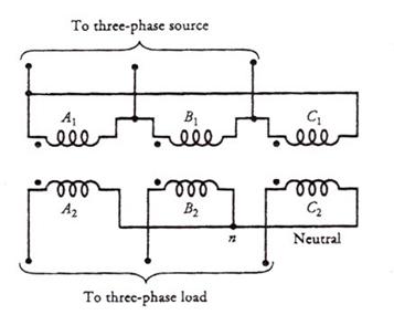
Figure 1.40 A D/Y-connected three-phase transformer.
Analysis of a Three-Phase Transformer
Under steady-state conditions, a single three-phase transformer operates exactly the same way as three single-phase transformers connected together. Therefore, in our discussion that follows we assume that we have three identical single-phase transformers connected to form a three-phase transformer. Such an understanding helps us to develop the per-phase equivalent circuit of a three- phase transformer.
We also assume that the three-phase transformer delivers a balanced load, and the waveforms of the induced emfs are purely sinusoidal. In other words, the magnetizing currents are not distorted and there are no third harmonics.
We
can analyze a three-phase transformer in the same way we have analyzed a
three-phase circuit. That is, we can employ the per-phase equivalent circuit of
a transformer. A D-connected
winding of a three-phase transformer can be replaced by an equivalent
Y-connected winding using D-to-Y transformation. If ![]() is the impedance in a D-connected
winding, the equivalent impedance
is the impedance in a D-connected
winding, the equivalent impedance ![]() in a Y-connected winding is
in a Y-connected winding is
 (1.42)
On
the other hand, if ![]() is the line-to-line
voltage in a Y-connected winding the line-to-neutral voltage
is the line-to-line
voltage in a Y-connected winding the line-to-neutral voltage ![]() is
is
 (1.43)
where the plus sign is for the negative phase-sequence (counterclockwise) and the minus sign is for the positive phase-sequence (clockwise).
The following examples show how to analyze a system of balanced three-phase transformers. Unless it is specified otherwise, we assume that the impressed voltages on the primary side follow the positive phase-sequence.
1.12 Instrument Transformers
Instrument transformers are designed to facilitate the measurements of high currents and voltages in a power system with standard but very accurate low-range ammeters and voltmeters. They also provide the needed safety in making these measurements, as the primary and the secondary windings are electrically isolated. Instrument transformers are of two kinds current transformers and potential transformers.
The Current Transformer
The current transformer, as the name suggests, is designed to measure high current in a power system. The primary winding has few turns of heavy wire, whereas the secondary has many turns of very fine wire. In a clamp-on type current transformer, the current-carrying conductor itself acts as a one-turn primary. The wiring arrangements for a wound primary and clamp-on current transformers are shown in Figure 1.47. It is evident from the figure that a current transformer is merely a well-designed step-up transformer. As the voltage is stepped up, the current is stepped down.
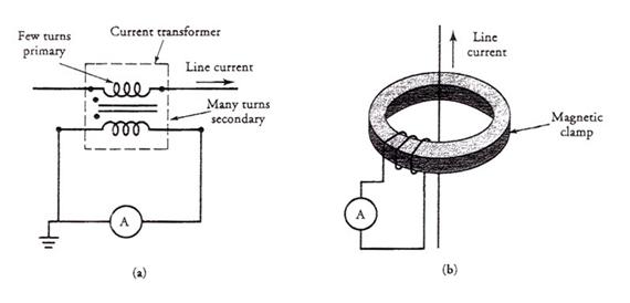
Figure 4.47 (a) Current transformer with wound primary. (b) Clamp-on type current transformer.
The low-range ammeter is connected across the secondary winding. Because the internal resistance of an ammeter is almost negligible compared with the winding resistance of the secondary, the ammeter can be treated as a short circuit. Therefore, the current transformers are always designed to operate under short-circuit conditions. The magnetizing current is almost negligible, and the flux density in the core is relatively low. Consequently, the core of a current transformer never saturates under normal operating conditions.
The secondary winding of a current transformer should never be left open. Otherwise, the current transformer may lose its calibration and yield inaccurate reading. The reason is that the primary winding is still carrying current, and no secondary current is present to counteract its mmf. The primary winding current acts like a magnetizing current and increases the flux in the core. The increased flux may saturate and magnetize the core. When the secondary is closed again, the hysteresis loop may not be symmetric around the origin but is displaced in the direction of residual flux in the core.
The increase in the flux causes an increase in the magnetizing current, which, in turn, invalidates its calibration. In addition, the primary current can produce excessive heat over a period of time and may destroy the insulation. Furthermore, the saturation may result in excessively high voltage across the secondary.
A current transformer is usually given a designation like 100:1. This simply means that if the ammeter measures 1 A, the current in the primary is 100 A. If an ammeter connected to a 100:5 transformer registers 2 A, the line current is 40 A.
The Potential Transformer
As the name suggests, a potential transformer is used to measure high potential difference (voltage) with a standard low-range voltmeter. A potential transformer, therefore, must be of the step-down type. The primary winding has many turns and is connected across the high-voltage line. The secondary winding has few turns and is connected to a voltmeter. The magnetic core of a potential transformer usually has a shell-type construction for better accuracy.
In order to provide adequate protection to the operator, one end of the secondary winding is usually grounded as illustrated in Figure 1.48.
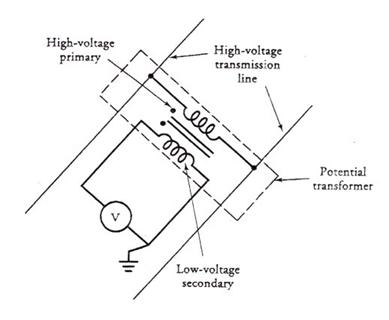
Figure 4.48 A potential transformer connected to measure high voltage with standard low-range voltmeter.
Since a voltmeter behaves more like an open circuit, the power rating of a potential transformer is low. Other than that, a potential transformer operates like any other constant-potential transformer. The a-ratio is simply the ratio of transformation. For example, if the voltmeter on a 100:1 potential transformer reads 120 V, the line voltage is 12,000 V. Some common ratios of transformation are 10:1, 20:1, 100:1, and 120:1.
The insulation between the two windings presents a major problem in the design of potential transformers. The primary winding may, in fact, be wound in layers. Each layer is then insulated in order to avoid insulation breakdown. Commonly used insulating materials in potential transformers are oil, oil-impregnated paper, sulfur hexafluoride, and epoxy resins.
|
Politica de confidentialitate | Termeni si conditii de utilizare |

Vizualizari: 5065
Importanta: ![]()
Termeni si conditii de utilizare | Contact
© SCRIGROUP 2024 . All rights reserved