Homework - Microwave Engineering

Homework - Microwave Engineering

Requirements

HW I.1 Locate the following load impedances terminating a 50Ω T-line:

(a)    Z_L = 0 (a short circuit),

(b)   Z_L = ∞ (an open circuit),

(c)    Z_L = 100 + j100 Ω,

(d)   Z_L = 100 - j100 Ω, and

(e)    Z_L = 50 Ω.

HW I.2 A 0.334λ - long Z_O = 50 Ω T - line is terminated in a load Z_L = 100 - j100 Ω. Use the Smith Chart to find:

(a)    Γ_L,

(b)   VSWR,

(c)    Z_in, and

(d)   the distance from the load to the first voltage minimum.

HW I.3 Suppose in Example 2.1 that the 50 Ω coaxial air line extends all the way from 0 cm scale location to the location of the termination. What is the shortest length this extension can be?

Solutions

HW I.1 For the graphical representations, see Figure 1 below. We know that Z_C = 50 Ω.

(a)    Z_L = 0 => see the blue color;

(b)    Z_L = ∞ (an open circuit) => see the red color;

(c)    Z_L = 100 + j100 Ω => the normalized impedance z_L = 2 + j2 Ω; see the magenta color;

(d)    Z_L = 100 - j100 Ω => the normalized impedance z_L = 2 - j2 Ω; we move on the Smith Chart in the clockwise direction; see the green color;

(e)    Z_L = 50 Ω => z_L = 1 Ω; we are now in the center of the Smith Chart; see the orange color.

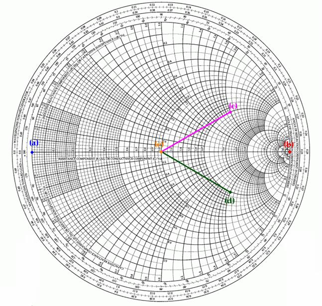
Figure 1. The representations on the Smith Chart for HW I.1

HW I.2

(a) Z_L = 100 + j100 Ω and Z_C = 50 Ω => the normalized impedance is z_L = 2 + j2 Ω; we now use the sub point (c) from exercise HW I.1.

In order to find | Γ_L | (the magnitude of the reflection coefficient), we have to measure the distance from the center of the Smith Chart to the point (c), and divide it to the radius of the big Smith circle; we obtain | Γ_L | = 0.62. The angle of the reflection coefficient is read from the graph: θ_Γ = 30^o.

For the graphical representation, see Figure 2 below:

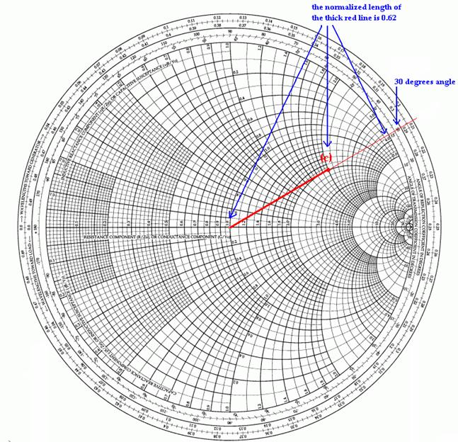
Figure 2. Graphical representation for determining Γ_L

(b) We now draw the constant - | Γ_L | circle. The voltage standing wave ratio VSWR can be determined by reading the value of r at the θ_Γ = 0^o crossing for the constant - | Γ_L | circle:

z = r = VSWR = 4.2

(c) We still use the constant - | Γ_L | circle. The starting point is at 0.208 λ. Adding the length of the line 0.334λ, we obtain 0.542λ; normalized to the interval (0 λ, 0.5 λ), we obtain 0.042λ. At this wavelength, we consider the intersection point with the constant - | Γ_L | circle => z_in = 0.24 + j0.26 Ω; de-normalizing, we obtain the input impedance:

Z_in = (0.24 + j0.26) x 50 Ω = 12 + j13 Ω.

For the graphical representation of (b) and (c), see Figure 3 below:

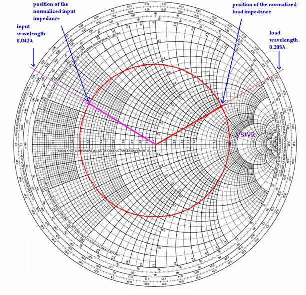
Figure 3. Graphical representation of the input impedance determination

d) We have: Z_L = 100 + j100 Ω and Z_C = 50 Ω => the normalized impedance is z_L = 2 + j2 Ω => we read on the Smith Chart 0.208 λ (from Figure 3). Considering the same scale as in Example 2.1, we have 30cm/λ. Thus, the distance from the load to the first voltage minimum is:

d = 0.208λ x 30 cm/λ = 6.24 cm.

HW I.3 At the given frequency of the signal, the coaxial air line should contain at least a minimum and a maximum; thus, the minimum length of the wire should be λ/2

=> d_min = 30 cm/λ x λ/2 = 15cm.