| CATEGORII DOCUMENTE |
| Asp | Autocad | C | Dot net | Excel | Fox pro | Html | Java |
| Linux | Mathcad | Photoshop | Php | Sql | Visual studio | Windows | Xml |
SELECT
Many developers spend their whole lives thinking that SELECT is the only SQL command in the FoxPro language-and with good reason. It's undoubtedly the most commonly used command and arguably the most useful. Why? Well, people generally put data into databases because they want to get it out later. While you can use the BROWSE command to view a table or set of tables, generally you will want to pull out only a subset of the data from a database. You can use SELECT to do so.
Sample databases
Before
I get started, I need to describe the tables used as examples in this chapter.
In most of this chapter, I'll use a pair of tables,
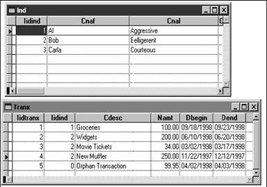
I'll use a different pair of tables for the discussion of outer joins, a feature added to Visual FoxPro's SQL implementation in version 5.0. While people and their associated transactions have all the elements needed for most SQL commands, outer joins have a couple of special aspects that are more easily explained through a different data set.
Basic SELECT syntax
A SQL SELECT command consists of about a half dozen clauses that specify which table or tables are being queried, which fields are being pulled from those tables, how to match up tables if more than one is used, which records from those tables are being selected (the record filter), and where to send the result (the destination). As with most things, this will get more involved as we explore the details, but here is the SELECT command in a nutshell.
In its most stripped-down form, a SQL SELECT command that pulls data from a single table consists of two essential clauses. The first clause-using the SELECT keyword- specifies what you are pulling out of the table, and the second clause-using the FROM keyword-specifies what table you are pulling the data from. Visual FoxPro has built-in defaults for the record filter and the destination if they are not provided. An example of the most trivial type of SELECT would be:
select * from TRANX
which will pull all the fields (denoted by the asterisk) from all the records in the TRANX table and display them in a browse window titled "Query." If the TRANX table is not opened, it will be opened automatically. It is important to note that SQL commands do not close tables after they finish with them.
Field lists
As we've seen, you can use the asterisk as shorthand to specify all fields in the table. The asterisk will pull all the fields in all the tables if the SELECT is using more than one table. You can also specify to select only certain fields by using a field list in place of the asterisk:
select iidTranx, dBegin, dEnd, nAmt from TRANX
This will pull only those four fields from the TRANX table and, again, display them in a browse window named Query.
If you are pulling fields from more than one table, you can use just the field name unless that name is present in more than one table. In this case, you need to precede the field name with the table alias. For example, if we were going to pull records from the Transaction table but also wanted the name of the individual to whom that transaction belonged to, we might also want to display the primary key values. And because the Individual table's primary key (iidind) is a foreign key in the TRANX table, it exists in both the Individual and Transaction tables. Thus, it is necessary to specify it, like so:
select
iidtranx, TRANX.iidind, dBegin, dEnd, nAmt, cNameIn ;from
(I'll discuss the WHERE clause in the "Multi-Table SELECTs" section below.) Forgetting the "TRANX" identifier before the iidind field after the SELECT keyword will result in this error message: "iidind is not unique and must be qualified."
Oftentimes, you will want to pull all the fields from one table but just a couple from another table. Instead of laboriously typing each field name, you can specify all the fields from one of the tables with the table alias and an asterisk, like so:
select
TRANX.*, cNameIn ;from
Even with a consistent naming scheme such as the one used in this book, field names are often terse and cryptic due to the fact that Visual FoxPro only allows them to be 10 characters long for tables that don't belong to a database. Accordingly, the result set of a SELECT may be hard to read with strange-looking column headings. You might wish to use alternate headings with the "AS" keyword:
select iidtranx as TRANS_ID, ;TRANX.iidind as IND_ID, ;dBegin as BEGIN_DATE, ;dEnd as END_DATE, ;nAmt as TRANS_AMT, ;cNameIn as DEPOSITOR ;
from
where TRANX.iidind = IND.iidind
Notice the indenting of this command. It would have been too long to fit on one line, but haphazard line breaks tend to cause more errors than a line that is "neatly" formatted. However, in order to indicate that the second through sixth lines are all part of the same clause, they are all indented an extra space. You'll see this same technique again when I explore multi-line WHERE clauses.
Depending on your personality and the amount of time you have to fine-tune things, you might want to indent the AS part of each phrase so they all line up. If you're having trouble with syntax errors and can't find "that one missing comma," this might be a helpful technique to hunt the errant typo:
select ;iidtranx as TRANS_ID, ;TRANX.iidind as IND_ID, ;dBegin as BEGIN_DATE, ;dEnd as END_DATE, ;nAmt as TRANS_AMT, ;cNameIn as DEPOSITOR ;
from
where TRANX.iidind = IND.iidind
You are not limited to field names in the fields list clause of a SELECT command. You can also use expressions and functions. Suppose you want to determine the number of days between the Begin and End dates of a transaction:
select ;
iidtranx as TRANS_ID, ;
dEnd - dBegin as TRAN_DIFF, ;
nAmt as TRANS_AMT ;
from TRANX
If you want to look up a surcharge based on the amount, you could use a UDF to return the surcharge amount beside the amount:
select ;
iidtranx as TRANS_ID, ;
dBegin as BEGIN_DATE, ;
dEnd as END_DATE, ;
nAmt as TRANS_AMT, ;
lupsur(nAmt) as SURCHARGE ;
from TRANX
If you do so, however, you should be aware of two things. First of all, using a UDF will dramatically slow down the SELECT, because no matter how you code it, it's going to be called for every record in the result set. And second, because of this, you'll want to optimize the living daylights out of the function-a savings of a tenth of a second will make a huge difference in a 40,000-record result.
It is important to note that SQL will do a lot of "behind the scenes" work, including opening up temporary tables, indexes, and relations. How and when these operations are done varies with how the SQL optimizer interprets the command. As a result, you cannot assume anything about the environment, such as the current work area, the names of the tables, or even which fields are currently being processed. The only guaranteed method of passing this information to a UDF is to do so through explicit parameters.
A number of SQL SELECT-specific functions (such as COUNT, SUM, and AVERAGE) do aggregate calculations on the result set. I'll discuss these in the "Aggregate functions" section later in this chapter.
Record subsets
More often than not, you won't want all of the records in the table to land in your result set. To filter out the records you don't want, use the WHERE clause. The WHERE clause is similar to the FOR clause in regular Xbase as far as functionality and basic syntax are concerned. A WHERE clause contains an expression, an operator, and a value. For instance, to select all records with a transaction amount over 100:
select ;iistranx as TRANS_ID, ;dBegin as BEGIN_DATE, ;dEnd as END_DATE, ;nAmt as TRANS_AMT ;
from
TRANX ;
where nAmt > 100
You can use multiple WHERE clauses by appending them with AND or OR keywords. This command will return all records with an AMOUNT of more than 100 AND whose value in the dBegin field is later than January 1, 1990:
select ;iidtranx as TRANS_ID, ;dBegin as BEGIN_DATE, ;dEnd as END_DATE, ;nAmt as TRANS_AMT ;
from
TRANX ;
where nAmt > 100 ;
and dBegin >
You are not limited to using fields in a WHERE clause that are also in the result set. For instance, you might just want the dates of the larger transactions:
select ;iidtranx as TRANS_ID, ;dBegin as BEGIN_DATE, ;dEnd as END_DATE ;
from TRANX ;where nAmt > 100
The WHERE clause is not limited to simple comparison operators. You can also select records where a column has values that fall in or out of a range, that match a pattern of characters, or that are found in a specific list of values. The BETWEEN operator allows you to select a range of values. This operator is inclusive-in this example, records with a Begin Date of 1/1 or 1/31 will be included in the result set:
select ;iidtranx as TRANS_ID, ;dBegin as BEGIN_DATE, ;dEnd as END_DATE, ;nAmt as TRANS_AMT ;
from
TRANX ;
where between(dBegin, , )
Most programmers are familiar with the asterisk (*) and question-mark (?) DOS wildcards that stand for "any number of characters" and "just one character." SQL uses the percent (%) sign to stand for "any number of characters" and the underscore (_) to represent just one character. One difference, however, is that the DOS asterisk ignores any characters placed after it, while the SQL percent sign does not. In addition, the SQL operator "like" is used with pattern-matching characters. For instance, this will find all records with the word "Visual" somewhere in the field cDesc:
select cDesc, dBegin, dEnd, nAmt ;
from TRANX ;
where cDesc like '%Visual'
And if the user typed "Visaul" a lot, you could use this command to look for records with any character in the fourth and fifth positions:
select cDesc, dBegin, dEnd, nAmt ;
from TRANX ;
where cDesc like '%Vis__l'
To test for a string that contains one of these wildcard values, precede the wildcard value with a literal character expression of your choosing, and then use the ESCAPE keyword to identify the literal character expression. This is difficult to imagine, so let's suppose our Description column in the TRANX table contains a percent sign. Searching for just those records that contain a percent sign somewhere in the Description field with a command like this would meet with a spectacular lack of success:
select cDesc, dBegin, dEnd, nAmt ;
from TRANX ;
where cDesc like '%%%'
(You'd end up with the entire table in the result set, right?) Instead, define a literal character such as the tilde (~) and then precede the character to search for with the literal:
select cDesc, dBegin, dEnd, nAmt ;
from TRANX ;
where cDesc like '%~%%' escape '~'
The first and third percent signs evaluate to "any number of characters" at the beginning or end of the string, and the tilde plus percent sign character pair evaluates to "the actual percent sign character in the Description field."
You can also test a column against a list of values. This list might take the form of a hand-typed string of discrete values, or of a result set of a second query. The second type is called a "sub-select" and will be covered in the "Outer joins" section later in this chapter. An example of the first type would be looking for rows where the Description was either a "Beginning," an "Ending," or a "Transitory" transaction:
select cDesc, dBegin, dEnd, nAmt ;
from TRANX ;
where upper(cDesc) in ('BEGINNING', 'ENDING', 'TRANSITORY')
You can also use the NOT
keyword to reverse the effect of an operator, such as BETWEEN, LIKE, or IN. For
example, the
select
cName, cTitle from
Like other commands in VFP, string comparisons in SQL are case-sensitive, so a WHERE condition that uses an expression like cTitle = "President" will catch only those records where the title was typed in proper case. All uppercase, lowercase, or mixed case (pRESIDENT) will be ignored. Because it's impossible to train users, and despite my best intentions I never manage to completely convert all data to a consistent state, I've found it safer just to test for the uppercase version of fields to constants also in uppercase.
However, there might be some titles where the word "manager" is not the entire title-and in fact might have several words surrounding it. So you could use a compound WHERE clause, like so:
sele cName, cTitle from
where uppe(cTitle) not in ('OWNER', 'PRESIDENT') ;
and upper(cTitle) not like '%MANAGER'
If you try this same command with an "OR" instead of an "AND", the entire table will be returned because, when a specific record matches one condition, it will not match the other- thus the entire WHERE clause returns a True value and the row will be included in the result set.
Note that filters you've set with other Visual FoxPro commands, such as SET FILTER TO, are completely ignored by the WHERE clause. However, the setting of SET DELETED is respected. In other words, records tagged for deletion will be ignored if SET DELETED is ON.
The WHERE clause can also be used to join two or more tables together. This is completely discussed in the "Multi-Table SELECTs" section later in this chapter.
Aggregate functions
You don't have to use SQL to return a collection of records. You might just want to find out "how many" records satisfy a given condition, or find out the highest, lowest, sum, or average value for a column. You can use one of SQL's aggregating functions to do so. The trick to remember here is that even though you are, say, summing values for a group of records, the result set is just a single record that contains the value you were calculating. For instance, to find the sum of the Amount field for all transactions that began in 1994:
select sum(nAmt) from TRANS ;where between(dBegin, , )
This will produce a result set of one record that contains the calculated amount. You can do several aggregate functions at the same time, as long as they are all for the same set of records:
select count(nAmt), sum(nAmt), min(nAmt), max(nAmt) from TRANS ;where between(dBegin, , )
Including fields that don't play into the aggregations will produce nonsensical results:
select cIDTr, count(nAmt), sum(nAmt) from TRANS ;where between(dBegin, , )
This query will place a value in the cIDTr field, but it won't have any meaning to the rest of the result set.
We'll be able to create a "subtotaling" report using these aggregate functions and a descriptive field in combination with the GROUP BY keyword. I'll discuss this next.
Subtotaling-GROUP BY
You've seen that it's possible to create a single record that contains an aggregate calculation for a query-for example, the total of all transactions between two dates. Oftentimes, however, you'd like subtotals as well-say, the total of all transactions for each individual in the system. Use the GROUP BY keyword to do so. The following command will create one record for all transactions in 1994 for each individual ID (cIDIn).
select ;
count(nAmt), ;
sum(nAmt) ;
from
TRANS ;
where between(dBegin, , ) ;
group by cIDIn
Internally, SQL creates a temporary table that contains all fields in the fields list as well as the grouping expression, but just for the records that satisfy the WHERE condition, like so:
nAmt, cIDIn
Obviously, there might be multiple rows in this temporary table for each individual ID. Then SQL performs the aggregation functions, creating a single row for each unique instance of the individual ID. If the grouping expression isn't one of the fields-list fields (in this case, it isn't), it simply isn't placed in the result set. Typically, however, you'd probably want to include the grouping expression or another identifier in the result set, or else you'd have a series of numbers with no descriptor-technically correct but useless in practice.
Multi-Table SELECTs
As powerful as SQL is,
it would be pretty useless if it only operated on a single table at a time.
However, multi-table SELECTs really bring out the power and elegance of using
SQL in your programs. When writing procedural code, it usually takes about a half-dozen
lines of code simply to identify the relationship between two files, and even
more code if a third or a fourth file is involved. And, as you know if you've
done it, the syntax and order of the commands is somewhat tricky and a nuisance
to keep straight. With SQL, however, joining two tables requires only an
additional WHERE clause. As you saw in a previous example, the following
command will automatically join two tables and pull the name of the individual
from the
select ;
iidtranx as TRANS_ID, ;
TRANX.iidind as IND_ID, ;
dBegin as BEGIN_DATE, ;
dEnd as END_DATE, ; nAmt as TRANS_AMT, ;
cNameIn
as DEPOSITOR ;
from
where TRANX.iidind = IND.iidind
This special WHERE clause, in which the parent key in one table is equated to the foreign key in the other table, is called a "join condition." If you name the keys to the various tables with a consistent scheme that makes writing the join condition simple, it's a painless operation to select data from multiple tables. However, there are three important points to remember about multi-table joins.
First, if you neglect the join condition, SQL
will attempt to match every record in one table with every record in the other
table; this is known as a Cartesian join. In other words, if TRANX has 100,000
records and
The second item to remember about joins is how SQL actually matches records. SQL will start from the child side of the relation and find the matching parent. If the parent has no children, the parent record will be left out of the result set. In our example, individuals without transactions will be left out of the result set in the above query. However, if you want all individuals matching a condition, regardless of whether they have transactions, you need to do an outer join, which will be discussed in detail in the "Outer joins" section later in this chapter.
The third warning about multi-table SELECTs concerns joining three or more tables. SQL is not designed to handle a join of one parent and two children. For example, an individual might have several transactions in the TRANX table, and also several phone numbers in the PHONES table. It is not possible to create a single simple SELECT command that will produce a result set that contains individuals with their transactions and their phone numbers at the same time. (You can do it with some advanced techniques, which will be discussed later.) If you try it, you will end up with a result set from the parent and one of the children-whichever has more records. The query might seem to work, but the answer created will be wrong.
Outer joins
As I mentioned a couple paragraphs earlier, an ordinary SQL join will match only records that have both a parent and a child. These are called "inner joins." If you want SQL to include records on one side or another that don't have a corresponding record on the other side, you need to create an "outer join."
In versions prior to VFP 5.0, you had to resort to a bit of trickery to make an outer join happen. Most SQL implementations use a NULL record to act as a "placeholder" for the records with missing children. With earlier versions of Fox, however, people actually created two queries-one that collects all the parents with children, and a second that collects all the parents without children-and then combined those two collections into a final result set.
With VFP 5.0 and later, true outer join support was available, but I'll discuss the two-query technique because you might run across existing applications that use it, and it can be useful elsewhere. The tables I'll use in the next few examples are shown in Figure 4.1.
The following query-yes, it's a long one-is the old way of combining two tables when you wanted to include all records regardless of if they had a child for every parent:
select ;cNaF as DEPOSITORF, ;cNaL as DEPOSITORL, ;dBegin as BEGIN_DATE, ;dEnd as END_DATE, ;nAmt as TRANS_AMT ;
from
where TRANX.iidind = IND.iidind ;
union all ;
select ;cNaF as DEPOSITORF, ;cNaL as DEPOSITORL, ;
as
BEGIN_DATE, ;
as END_DATE, ;
00000.00
as TRANS_AMT ;
from
where iidind not in ;
(select distinct iidind from TRANX)
The first query (everything up to the UNION clause) isn't too bad-it just pulls all individuals with transactions. The second query, however, is much more complex and actually does two things. The subselect query in the WHERE clause puts together a list of all the individuals with transactions-by finding their foreign keys. Then the main SELECT command pulls all individuals where the individual ID is not in the subquery list-in other words, those individuals without transactions.
The UNION keyword
requires that the structures of the two result sets must be identical. Because
the
One final note about this outer join methodology: SQL always matches empty records and will place those records in the result unless you guard against it by eliminating empty records with an additional WHERE clause, like so:
select ;cNaF as DEPOSITORF, ;cNaL as DEPOSITORL, ;dBegin as BEGIN_DATE, ;dEnd as END_DATE, ;nAmt as TRANS_AMT ;
from
where TRANX.iidind = IND.iidind ;
and not empty(dBegin) ;
union all ;
select ;cNaF as DEPOSITORF, ;cNaL as DEPOSITORL, ; as BEGIN_DATE, ; as END_DATE, ;00000.00 as TRANS_AMT ;
from
where iidind not in ;
(select distinct iidind from TRANX) ;
and not empty(dBegin)
Now that I've discussed the old way it was done, you'll undoubtedly have a much fuller appreciation for the outer join syntax. Before getting into the nuts and bolts of all the keywords, here's what a simple outer join looks like:
sele ind.cnaf, ind.cnal, tranx.dBegin, dEnd, nAmt ;
from
tranx ;
full outer join
on tranx.iidind = ind.iidind
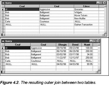
The result of the outer join is shown in Figure 4.2.
Note that there are six
records-Al's one transaction, Bob's three transactions, and two more-one for
Carla, even though she didn't have any transactions, and one for the orphan
transaction. If a regular join had been performed here, the result set would
have had only four records: one for Al and three for Bob. The
While technically correct, we can set this up to look better. Here's the same outer join with friendly replacements for .NULL., using the NVL function:
select nvl(ind.cnaf, 'No first name'), nvl(ind.cnal, 'No last name'), ;nvl(tranx.cdesc, 'No transaction') ;from tranx ;
full
outer join
on tranx.iidind = ind.iidind
Let's examine the syntax:
select <field> from table1 join table2 on t1.field = t2.field
You'll see that there is no WHERE clause at all-it's now been relegated to simply performing filtering, as it should have been all along. (WHERE will still function as a tool to join two tables, preserving the functionality of legacy code, but such a use is now outdated.)
The new keyword is JOIN, and it has four variants:
. . JOIN (inner join)
. . RIGHT JOIN (right outer join)
. . LEFT JOIN (left outer join)
. . FULL JOIN (full outer join)
Using JOIN without a preceding qualifier simply performs a join between two tables in the same way that WHERE used to-the result is an "inner" join, one where records without matches are ignored. The qualifiers "RIGHT" (or "RIGHT OUTER"), "LEFT" (or "LEFT OUTER"), and "FULL" (or "FULL OUTER") now allow you to dictate how records without matches are handled.
The FULL OUTER JOIN is obvious-records without matches on both sides of the join are also included. However, the RIGHT and LEFT might not be as intuitive. There may be times when you only want matches from one side of the relationship-for example, individuals with, and without, transactions-but you don't want orphaned transactions (those that somehow were entered or kept in the database without a corresponding individual record).
The following SELECT produces all individuals, with and without transactions:
select nvl(ind.cnaf, 'No first name'), nvl(ind.cnal, 'No last name'), ;
nvl(tranx.cdesc, 'No transaction') ;
from
left outer join tranx ;
on tranx.iidind = ind.iidind
The following SELECT does the opposite: transactions with and without individuals:
select nvl(ind.cnaf, 'No first name'), nvl(ind.cnal, 'No last name'), ;
nvl(tranx.cdesc, 'No transaction') ;
from
right outer join tranx ;
on tranx.iidind = ind.iidind
Let's examine these examples in more detail.
You'll note that, along with the OUTER JOIN keyword, an ON <expression> construct is used. This logical expression describes how the two tables are joined. The qualifier of the JOIN simply describes which side will contain records that don't have matches on the opposing side. Thus, a SELECT command like:
from A right outer join B
will grab all records from B, whether or not they have matches in A. You could produce the same effect by using a LEFT JOIN and reversing the order of the tables, like so:
from B left outer join A
I typically keep the "parent" table on the left side of the JOIN expression, and have either children or lookup tables on the right side. There's no technical reason for doing so-I just find it easier to visualize the result set in my mind.
Now that I've dissected a two-table join, it's time to move on to joins involving three or more tables. Before doing so, I need to mention that there are two fundamental rules involved in an outer join. First, you can't reference a table in the ON clause until it's been opened in a JOIN. While this can't happen in a two-table join constructed as shown in the preceding example, it's easy to do in joins involving three or more tables, and I'll come back to this rule. The second rule is that each JOIN/ON combination creates an intermediate result, which is then used in the rest of the JOIN.
To illustrate these rules, suppose you were joining a parent table, A, with two lookup tables, T1 and T2, both of which had foreign keys in A. You would need to define the A - T1 join, and describe the ON condition for A - T1, before getting A involved with T2, like so (I've eliminated the field list and the actual field names from the ON conditions for simplicity's sake):
from A join T1 on A = T1 ;join T2 on A = T2
Syntax like this wouldn't work:
from A join T1 join T2 ;on A = T1 on A = T2
The result of the A - T1 join couldn't be joined with T2 because the A - T1 ON condition hadn't been found by the SQL parser.
With that theory behind us, let's look at a typical use for an outer join: including the values from a lookup table in a join, whether or not the parent table always used those values.
As an example, suppose
our individual table recorded information such as personality type, hair color,
and type of car driven. However, instead of storing values like "BLONDE" and
"CLUNKER" in the
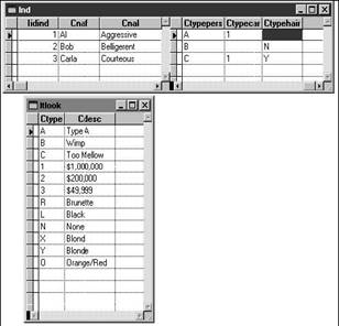
The goal is a list of the individuals, together with their personal attributes, but a simple join won't work because some of the attributes are missing. As with many things, it's best to start slowly and build up: If you try to create a five-table join with a variety of qualifiers, you're dooming yourself before you begin.
select
ind.cnaf, ind.cnal, itlook.cdesc ;from
This is pretty ugly-a bunch of .NULL.'s floating around. Try again:
select
nvl(ind.cnaf, 'No first name'), nvl(ind.cnal, 'No last
name'), ;itlook.cdesc ;from
This still isn't what you want, because it will include records for every value in the lookup table, whether or not they are used. Clearly, a LEFT JOIN will just grab the individuals:
select
nvl(ind.cnaf, 'No first name'), nvl(ind.cnal, 'No last
name'), ;itlook.cdesc ;from
However, this isn't enough-you want all of the attributes. Getting all three lookup values in one step is going to be too complex, so I'm just going to address a second attribute for now.
To do so, you have to
grab personality types from the lookup table and join them with the
from A join LOOKUP LOOK1 ;on A = LOOK1 ;join LOOKUP LOOK2 ;on A = LOOK2
You'll see that the reference to the lookup table is followed once by the expression LOOK1, which is the alias that will be used in that join, and then by the expression LOOK2, which is the alias that will be used in the second join. Now that you see what the basic idea is, here's the real code:
select
nvl(ind.cnaf, 'No first name'), nvl(ind.cnal, 'No last
name'), ;look1.cdesc as perstype, look2.cdesc as cartype ;from
on
ind.ctypepers = look1.ctype ;
join itlook look2 ;
on ind.ctypecar = look2.ctype
The results for this and the next two queries
are shown in Figure 4.4. This first example won't perform quite as
expected; because it's a simple join, only records that exist in both the
select
nvl(ind.cnaf, 'No first name'), nvl(ind.cnal, 'No last
name'), ;look1.cdesc as perstype, look2.cdesc as cartype ;from
on
ind.ctypepers = look1.ctype ;
join itlook look2 ;
on ind.ctypecar = look2.ctype
This one doesn't do much
better, because it's only doing one LEFT JOIN between
select
nvl(ind.cnaf, 'No first name'), nvl(ind.cnal, 'No last
name'), ;look1.cdesc as perstype, look2.cdesc as cartype ;from
on
ind.ctypepers = look1.ctype ;
left join itlook look2 ;
on ind.ctypecar = look2.ctype
Here's where you will
strike gold-selecting every record from the
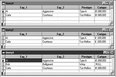
Note that the first two SELECTs didn't work, even though all three individuals had matches in the lookup table for personality type. Bob didn't show up because he didn't have a match in the Cartype field.
It's time to add the
third lookup table. Instead of just giving you the "answer," let's look at
several possible permutations and discuss why they won't work. The following
SELECT command will produce the error "Alias LOOK1 not found" because the first
ON clause references both
select ind.cnaf, ind.cnal, ;ind.ctypepers, look1.cdesc as perstype, ;
ind.ctypehair, look3.cdesc as hairtype, ;
ind.ctypecar, look4.cdesc as cartype ;
from
itlook look3 right outer join ;
itlook look1 right outer join ;
on
look1.ctype = ind.ctypepers ;
on look3.ctype = ind.ctypehair ;
on look4.ctype = ind.ctypecar
This next attempt
produces the error "Alias LOOK3 not found" because LOOK1 and LOOK4 have been
moved, but the second ON clause references LOOK3 and
select ind.cnaf, ind.cnal, ;ind.ctypepers, look1.cdesc as perstype, ;ind.ctypehair, look3.cdesc as hairtype, ;ind.ctypecar, look4.cdesc as cartype ;
from
itlook look3 right outer join ;
itlook look1 right outer join ;
on
look4.ctype = ind.ctypecar ;
on look3.ctype = ind.ctypehair ;
on look1.ctype = ind.ctypepers
Moving LOOK3 and LOOK1 so that the third ON clause references LOOK3, which is opened last, makes everything click:
select ind.cnaf, ind.cnal, ;ind.ctypepers, look1.cdesc as perstype, ;ind.ctypehair, look3.cdesc as hairtype, ;ind.ctypecar, look4.cdesc as cartype ;
from
itlook look3 right outer join ;
itlook look1 right outer join ;
on
look4.ctype = ind.ctypecar ;
on look1.ctype = ind.ctypepers ;
on look3.ctype = ind.ctypehair
Another type of multi-table outer join involves many-to-many relationships. For example, table A can have zero or more matching records in table B, and the same goes for B-it can have zero or more matching records in table A. To accommodate this requirement, a third table, AB, is used to hold keys for both tables for every instance of a match. Getting an outer join to work in this situation is a little tricky.
Suppose you have two tables, PART and IMAGE. The PART table has records for every part stocked in the machine shop, and IMAGE has records for every blueprint in the machine shop. A single PART might not have a blueprint (because it's purchased from outside, or because the blueprint has been lost). A PART might also have a single blueprint, or it might have multiple blueprints if it's a complex part. Furthermore, the same blueprint might be used for more than one part (two parts might differ only in material, color, or dimension, thus allowing the same blueprint to be used for each). Thus, the PARTIMAGE table contains keys from both the PART and IMAGE tables.
In this example, all records in PART will show up in the result set. Remember that the join table PARTIMAGE might have zero, one, or more IMAGE records for any specific record in PART. Thus, for a given record in PART, the result set might have a single record populated with .NULL. (indicating that there is no match in IMAGE-no blueprint exists), or one or more records from PART, indicating one or more matches (blueprints) for that part.
select ;
nvl(cNoPart, 'NO PART') as PartNumber, PART.cdepm as PartDesc, ;
nvl(IMAGE.cnaimage, 'NO IMAGE JACK') as ImageName ;
from IMAGE full outer join PARTIMAGE ;
on PARTIMAGE.iidimage = IMAGE.iidimage ;
full outer join PART ;
on PART.iidpart = PARTIMAGE.iidpart
Controlling the result set: destination
So far we've just worked with producing a result set, and "let the records fall where they may." However, we often want to do something special with the results of our query. For instance, we might want to order the result set in a particular way or use a second SELECT command on the contents of the result set.
You can send the results of a SELECT command to several different destinations. As you've seen, by default, Visual FoxPro uses a browse window named Query as the destination. You can specify one of three destinations for the output of a query: an actual table, a temporary table (located in memory) called a cursor, or an array.
The first destination is an array. This is useful for small result sets, such as a lookup table that will populate a combo box or list box on a form. It is also useful when you are using a SQL command to perform an aggregate function such as COUNT or SUM. More overhead and maintenance is necessary to place this information into a table or a cursor, and its size doesn't impact memory to any practical significance.
You need to remember that if the result set is empty, the array won't be created at all. You can use the _tally system variable to determine if the result set was empty. For instance, the following program code will place a value into the memory variable nTranSum, regardless of whether there were any qualifying records:
select ;
sum(nAmt) ;
from TRANX ;
where between(dBegin, , ) ;
into array aTranSumif _tally = 0
m.nTranSum = 0 else
m.nTranSum = aTranSum[1]endif
It looks like a bit more work, but using this construct as a standard practice will save you a lot of headaches and debugging in your programming.
The second destination is a table. If the result set of the query is going to be large (to preclude the use of an array) or if you need the result set to "hang around awhile," you'll want to send the result set to a table. This option actually creates a .DBF file (a free table) on disk that can be edited, modified, and otherwise treated like any other table. Note that this table will be created without warning if the setting of SET SAFETY is OFF, regardless of whether or not the table already exists, or whether it's even open in another work area.
The third destination is a cursor. We've been using the term "result set" to refer to the collection of records created by the execution of a SELECT command. While Visual FoxPro is "record oriented" in that we can move from record to record as we desire, other languages that use SQL do not have this capability and can only address a block of records as a single entity. As a result, all SQL operations are oriented toward manipulating this "set of records." They refer to this block of records as a "cursor," which stands for CURrent Set Of Records. A cursor is a table-like structure held in memory; it overflows to disk as memory is used up. In some cases, such as queries that essentially just filter an existing table (in other words, no calculations or joins), Visual FoxPro opens a second copy of the table in another work area and then applies the filtering condition to present a different view of the table as the query requests it.
Cursors have two advantages. First, they are fast to set up, partly because of the possible filtering of an existing table, and also because of their initial creation in RAM. Second, maintenance is greatly reduced, because when a cursor is closed, any files on disk created due to RAM overflow are automatically deleted.
Controlling the result set: ORDER BY
Records in a result set are presented in random order unless you use the ORDER BY keyword to control the order. Unlike indexes, which present a different view of the records but don't change the physical position, ORDER BY actually positions the records in the order specified by the ORDER BY field list.
You can use field names or the number of the position of the column in the field list. The latter option is useful when using functions that create columns with an unknown name. The default order is ascending, but you can override it by using the DESCENDING keyword.
Here's how to sort a result set by "transaction-begin date" and then by transaction amount within a single transaction-begin date:
select ;
cDesc as DESCRIPTION, ;
dBegin as BEGIN_DATE, ;
dEnd as END_DATE, ;
nAmt as TRANS_AMT ;
from
TRANX ;
order by dBegin, nAmt
To sort the result set of a GROUP BY SELECT command by the summed amount, use the column number of the aggregate function:
select ;
iidind, ;
count(nAmt), ;
sum(nAmt) ;
from TRANX
;
where between(dBegin, , ) ;
group by iidind ;
order by 3
Controlling the result set: DISTINCT
In cases where we are selecting a subset of the available fields in the source (either table or tables), it is possible to end up with a number of identical records. For instance, the Company table might contain multiple branches of the same company with different addresses but the same company name. If we want a list of all the companies in the table, we wouldn't necessarily want multiple copies of the same company name. The DISTINCT keyword eliminates all but one instance of duplicate records in the result set.
This is an important point: The DISTINCT keyword operates on the result set, which means just those fields in the result set, regardless of whether or not other fields in the original record would make two records in the result unique. This can be handy for determining values to use to populate a lookup table, for instance. Another reason to use the DISTINCT keyword is to find instances of typos in free-form text fields. For example, if the user has typed "Visual FoxPro", "Visaul Foxpro", and "Visual PoxFro" in a field, a SELECT command of this sort would identify those errors. You would need to use a second SELECT command to find those records containing "Visaul FoxPro", of course. The syntax of the command to create a list of all types of transactions from the TRANX table would look like this:
select distinct ;
cDesc as DESCRIPTION ;
from TRANX
In many cases, you will find you can use a GROUP BY SELECT command in place of the DISTINCT keyword-it's considerably faster. The same query with a GROUP BY clause would look like this:
select cDesc as DESCRIPTION ;
group by cDesc;
from TRANX
Controlling the result set: HAVING
The SQL SELECT command has another keyword that many programmers confuse with the WHERE keyword: HAVING. While it sounds like it would perform the same function, and, in fact, will do so, there is an important difference between WHERE and HAVING. While WHERE operates as a filter on the table to produce a filtered result set, HAVING operates on the result set to filter out unwanted results. For example, suppose the result set consisted of subtotals of transactions for multiple individuals, but we only wanted to see the individuals with high subtotal numbers. HAVING would enable us to weed out the "low subtotal" folk, like so:
select ;count(nAmt), ;sum(nAmt) ;
from
TRANX ;
where between(dBegin, , ) ;
group by cIDIn
having sum(nAmt) > 1000
Note that the function or expression in the HAVING clause does not have to be the same as in the fields list. For instance:
select ;count(nAmt), ;sum(nAmt) ;
from
TRANX ;
where between(dBegin, , ) ;
group by iidind
having avg(nAmt) > 640
Again, HAVING will produce the same results as WHERE, but it is not Rushmore optimizable and, as a result, will take considerably longer than WHERE in any but the most trivial of SELECTS. As a result, you should limit your use of HAVING with GROUP BY selects, because HAVING will work on the result set, but WHERE won't. HAVING, as opposed to WHERE, gives you the ability to winnow the results of a GROUP BY SELECT command.
|
Politica de confidentialitate | Termeni si conditii de utilizare |

Vizualizari: 1494
Importanta: ![]()
Termeni si conditii de utilizare | Contact
© SCRIGROUP 2025 . All rights reserved