| CATEGORII DOCUMENTE |
| Bulgara | Ceha slovaca | Croata | Engleza | Estona | Finlandeza | Franceza |
| Germana | Italiana | Letona | Lituaniana | Maghiara | Olandeza | Poloneza |
| Sarba | Slovena | Spaniola | Suedeza | Turca | Ucraineana |

Technical Graphics and Data Analysis in Windows
|
|
The Peak Fitting Module
Microcal Software, Inc.
1 - Introduction to the PFM
Data from chromatographic, spectroscopic, chemical, and pharmaceutical analyses usually have peaks. Researchers need to find suitable models and parameters in order to accurately determine and predict peak area and positions. Various data analysis techniques have been developed in the past to facilitate this process. The most practical is nonlinear least-squares curve fitting. This method can quickly and accurately determine suitable models and their parameters. The PFMTM module, as an addition to OriginTM, uses the nonlinear least-squares curve fitting method to fit functions to data to find various parameters and generate statistical results.
The PFM module is primarily designed to analyze data with many peaks. The kernel of the module is the Levenberg-Marquardt nonlinear least-squares curve fitter. Users can easily find parameters, given appropriate models for data. Many other data analysis routines are also included, such as statistical analyses. Most importantly, the PFM works inside the Origin system which provides graphing and analysis tools. Origin also has other optional add-on modules such as the data acquisition system modules which allow users to streamline their routine research work in an integrated environment.
Do not use Origin's standard fitting if you are using the PFM module. Conflicts might result.
Before installing the PFM module, you must install Origin. For Origin installation instructions, refer to the Origin Users Manual if you have Origin 4.1, or the Getting Started Booklet if you have Origin 5.
Perform the following steps to install the PFM module:
1. Start Microsoft Windows.
2. Quit all Windows programs.
3. Insert the PFM module disk in the available floppy drive (A: or B:).
4. In Windows 95 or Windows NT 4.0, select Run from the Start menu. In Windows 3.1, select File:Run from the Program Manager menu bar.
5. Type A:SETUP (or B:SETUP).
6. Click OK to close the dialog box and begin the installation program.
The installation program adds a PFM icon to the Microcal Origin window. The PFM icons command line includes two switches following the Origin executable file: -a pfm -tw pfm.
1.1 PFM Module Structure
The PFM module is an add-on module to Origin. Like other Origin modules, it consists of templates, scripting methods and properties, and a Dynamic Link Library. As a part of the integrated environment of Origin, it is compatible with all of the features and capabilities of Origin.
In order to use this module, you need to have a minimum amount of experience with Microsoft Windows and Origin. If you are not an experienced Origin user, review the Origin User's Manual and use the samples provided with the Origin package.
Origin's scripting capabilities can be used for customization. The LabTalk scripting language is a full-featured macro-type language that allows you to program your own control structures. The PFM module adds a new set of methods, properties and templates to fulfill most users peak fitting needs.
You can create custom templates. Do NOT alter a PFM template while fitting. Instead, exit and re-open Origin. Open the template by selecting File:Template:Open Graph Template or Open Worksheet Template in Origin 4.1, or File:New in Origin 5. Alter the worksheet or graph window according to your needs, then save it by selecting File:Template:Save As in Origin 4.1 or File:Save Template As in Origin 5, and typing in a name for the new template. In later peak fitting sessions you can use your customized template in two ways:
Open Origin with the command line Origin Executable -a pfm -tw worksheet_template -tp graph_template. Origin will use the specified templates as the defaults for that session. You do not need to include the .otw or .otp file extensions in the template names. For example: origin50.exe -a pfm -tw MyWks -tp MyPlot. For more information on command line switches, see the Origin User's Manual.
From inside Origin, open your template by selecting File:Template:Open Graph Template or Open Worksheet Template in Origin 4.1, or File:New in Origin 5. You can use a template opened in this way in the same way as a default template.
It is possible to change the default PFM template by selecting File:Template:Save in Origin 4.1, or File:Save Template As in Origin 5. However, this will over-write the original template. The only way to regain the original PFM template is to re-install the PFM.
1.2 Tutorial
This lesson is designed to help you master the PFM module. A sample dataset with four Gaussian peaks provided with the PFM disk is used in this example.
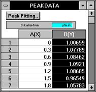
Start Origin by double-clicking on the Peak Fitting Module
icon. A worksheet named Data1 opens with a ![]() button. Import the sample data file PEAKDATA.DAT from
the Origin directory by selecting File:Import:ASCII
and clicking on the file name. The
PEAKDATA.DAT file contains two columns, A and B. These dataset names are peakdata_a and peakdata_b (WksName_ColName). We assume that the former is time (X values)
and the latter is amplitude (Y values).
We are going to fit the Y values to the Gaussian model. To do this, we start by clicking on the B(Y)
column heading to highlight the Y column.
Press the
button. Import the sample data file PEAKDATA.DAT from
the Origin directory by selecting File:Import:ASCII
and clicking on the file name. The
PEAKDATA.DAT file contains two columns, A and B. These dataset names are peakdata_a and peakdata_b (WksName_ColName). We assume that the former is time (X values)
and the latter is amplitude (Y values).
We are going to fit the Y values to the Gaussian model. To do this, we start by clicking on the B(Y)
column heading to highlight the Y column.
Press the ![]() button. A graph window named PFMPlot is opened. During this process, the configuration file
EASYPEAK.CNFis read in and the PFM is properly
initialized. (To create a custom
initialization file, see page 21.)
button. A graph window named PFMPlot is opened. During this process, the configuration file
EASYPEAK.CNFis read in and the PFM is properly
initialized. (To create a custom
initialization file, see page 21.)
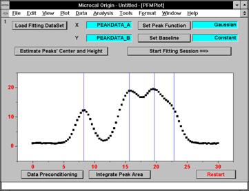
The Phase 1 window appears as follows. There are several objects in the window.
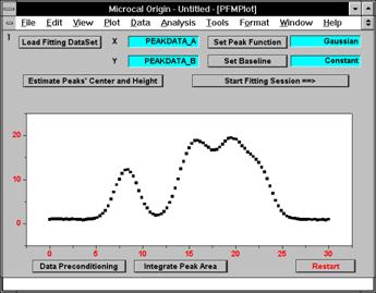
Loading the fitting datasets
To the right side of the ![]() button, the proper
fitting datasets (peakdata_a, peakdata_b) are already displayed in
two fields. If you have other fitting
datasets to use, you can load them by pressing the
button, the proper
fitting datasets (peakdata_a, peakdata_b) are already displayed in
two fields. If you have other fitting
datasets to use, you can load them by pressing the ![]() button. This action opens the Assign Fitting Dataset
dialog box. The Available DataSets list
box displays all Y datasets in the current project. To replace the dataset listed in the Y
Fitting DataSet list box, click on the desired dataset in the Available
DataSets list box. The Assign Fitting
Dataset dialog box respects column associations in the worksheet. Thus, the X Fitting DataSet list box automatically updates with the (correct)
associated X dataset for a given Y Fitting DataSet. This is also the case if the worksheet
contains multiple X columns.
button. This action opens the Assign Fitting Dataset
dialog box. The Available DataSets list
box displays all Y datasets in the current project. To replace the dataset listed in the Y
Fitting DataSet list box, click on the desired dataset in the Available
DataSets list box. The Assign Fitting
Dataset dialog box respects column associations in the worksheet. Thus, the X Fitting DataSet list box automatically updates with the (correct)
associated X dataset for a given Y Fitting DataSet. This is also the case if the worksheet
contains multiple X columns.
For this tutorial, you should use the datasets from the PEAKDATA.DAT ASCII file.
Setting the peak and baseline functions
The default fitting function is the Gaussian function. You can choose other functions by pressing
the ![]() button. If you need to set a different fitting
function for each peak, you can do it in the next phase. For this tutorial, you should use the
Gaussian function.
button. If you need to set a different fitting
function for each peak, you can do it in the next phase. For this tutorial, you should use the
Gaussian function.
Similarly, the baseline defaults
to the Constant function, i.e., a horizontal straight line (a vertical
offset). You can choose other baseline
functions by pressing the ![]() button. For this tutorial, you should use the
Constant function.
button. For this tutorial, you should use the
Constant function.
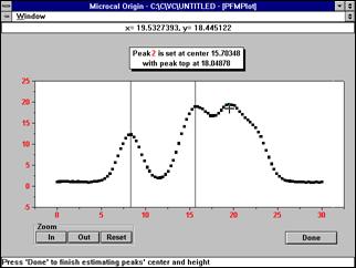
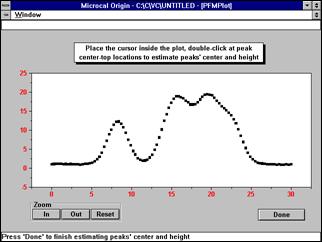
Estimate the peaks' center and height
Estimate
the peaks center and height by pressing the ![]() button. After this button is pressed, a new window
appears as follows. There are four peaks
in this example. The peak top-centers
are roughly located at the white circles.
Double-click from left to right at these circles. Each double-click gives a rough estimation of the height and center
of a peak. After each double-click, a
vertical peak-center-line is drawn. The
peak center line can be dragged to any position once it is created. Click on the
button. After this button is pressed, a new window
appears as follows. There are four peaks
in this example. The peak top-centers
are roughly located at the white circles.
Double-click from left to right at these circles. Each double-click gives a rough estimation of the height and center
of a peak. After each double-click, a
vertical peak-center-line is drawn. The
peak center line can be dragged to any position once it is created. Click on the ![]() button to stop.
button to stop.
![]()
![]()
![]()
![]()
![]()
![]()
![]()
Now the window is switched back to the Phase 1 window, with four peak-center-lines.
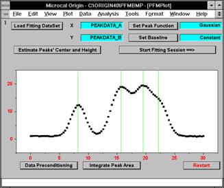
Data preparation prior to fitting
Prior to beginning the fitting, two operations are available for use on the data plot: preconditioning and integration to find the peak areas.
A preconditioning method may be selected interactively at run-time, or saved in an initialization file to be run automatically when new data is loaded into the PFM.
To access the interactive preconditioning methods in the
Phase 1 window, press the  button.
This action opens the Precondition Fitting DataSet dialog box. For information on this dialog box, see page 31.
button.
This action opens the Precondition Fitting DataSet dialog box. For information on this dialog box, see page 31.
The PFM provides an option to
find the area of your peaks by numerical integration of the data (via the
trapezoidal rule), in addition to using the Levenberg-Marquardt algorithm to
find the area parameter of your model function.
To integrate to find the peak areas, press the ![]() button (before integrating, you must estimate
the peaks' center and height). The PFM
determines the boundaries between peaks and marks them with red lines which you
may then click and drag. When you are
satisfied with the boundary positions, click on the
button (before integrating, you must estimate
the peaks' center and height). The PFM
determines the boundaries between peaks and marks them with red lines which you
may then click and drag. When you are
satisfied with the boundary positions, click on the ![]() button.
The PFM generates a worksheet named Area which contains the following
columns:
button.
The PFM generates a worksheet named Area which contains the following
columns:
|
Field Name: |
Description: |
|
PeakNum |
Ordinal number of peak. |
|
AreaInteg |
Area of peak by integrating data. |
|
AreaIntegP |
Area expressed as % of total. |
|
CenterSet |
X value where center was set. |
|
CenterMax |
X value where max occurs. |
|
MaxHeight |
Max Y value of this peak. |
|
CenterGrvty |
X value of peak center of gravity. |
|
Variance |
To return to the Phase 1 window,
press the ![]() button.
button.
Starting the fitting
Press the ![]() button to start peak fitting analysis and
enter the Phase 2 window.
button to start peak fitting analysis and
enter the Phase 2 window.
Note: pressing the ![]() button will
reinitialize the PFM and discard all parameters.
button will
reinitialize the PFM and discard all parameters.
The Phase 2 window is shown below. Most analyses are performed in this phase.
![]()
![]()

![]()
![]()
![]()

![]()
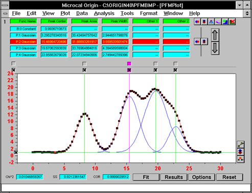
The upper part of the Phase 2 window displays the values of the parameters, which are modified in the fitting process to give an accurate fit. They are initialized according to the peaks centers and heights, as estimated in the previous phase.
Press the ![]() button to perform up to ten rounds of
nonlinear curve fitting. A red curve
named FitFunc_Fit is generated
according to the current parameter values.
However, you can do much more in this phase. Examine each callout in the above picture to
determine the use of each object. Return
to Phase 1 by pressing the
button to perform up to ten rounds of
nonlinear curve fitting. A red curve
named FitFunc_Fit is generated
according to the current parameter values.
However, you can do much more in this phase. Examine each callout in the above picture to
determine the use of each object. Return
to Phase 1 by pressing the ![]() button.
button.
Controlling fitting parameters
You can manually edit parameters by double-clicking on the parameters as shown in the picture. The Edit Fitting Parameters dialog box opens, which allows you to interactively control the parameters. From this dialog box, you can assign new values to parameters, fix parameters to set values, and limit parameters to within certain desirable ranges.
You can fix a parameter to a set value by clearing the check box on its left. This may help stabilize the PFM during fitting iterations. You can set a lower and an upper bound for each parameter. There are three types of constraints: internal bounds, user-set bounds and general linear constraints. For some parameters, internal bounds are already set properly. For example, the area of a peak is set to be greater than zero. Upper and lower bounds for the peak centers are reset to preserve their original order throughout fitting iterations. However, user-set bounds always take precedence, so if the user sets bounds for a parameter, its internal bounds will be invalid.
Controlling peak centers
You can drag the peak-center-lines to adjust peak center positions. The lower of the two check boxes above each peak-center-line is the peak center control. The centers of peaks with a checked peak center control can be modified during fitting iterations. The first parameter of a peak fitting function is always the peak center. The peak center check box in the upper-left corner of the graph controls the centers of all peaks. If checked, all peak centers can be modified during fitting iterations.
Fixing width for all peaks
The PFM allows you to force peaks to have equal width. The upper check box above the peak-center-line is the peak-width control. All peaks with checked width boxes are forced to have the same width. The upper-left check box controls the width of all the peaks.
Adding and removing peaks
The PFM provides buttons to add and delete peaks in the Phase 2 window without restarting the fitting session.
To add new peaks by setting new center tops, press the ![]() button.
This button re-opens the graph window used to estimate the peaks' center
and height (see page 12).
button.
This button re-opens the graph window used to estimate the peaks' center
and height (see page 12).
To delete the currently highlighted peak in the Phase 2
window, press the ![]() button.
button.
Resetting fitting functions
Although the peak fitting function
defaults to Gaussian, you can set it to another function. If you want to set the same function for all
of the peaks, press the ![]() button.
If you want to set a different function for each peak, click on the
function name, e.g., P:4 Gaussian for peak 4.
button.
If you want to set a different function for each peak, click on the
function name, e.g., P:4 Gaussian for peak 4.
You can change the baseline function by pressing the ![]() button. Alternatively, click on the baseline function
name in the Phase 2 window.
button. Alternatively, click on the baseline function
name in the Phase 2 window.
Note: Auto-initialization is always performed if any fitting function is set or reset. However, you need to provide initial values for the parameters of the user-defined baseline function.
Creating fitted curves
You can create a fitted curve for
each peak with or without the baseline.
These curves are called peak function plots. Pressing the ![]() button on the
six-button bar (at the top-right corner of the window) creates a peak function
plot for all peaks. The
button on the
six-button bar (at the top-right corner of the window) creates a peak function
plot for all peaks. The ![]() button on the moving
two-button bar creates a plot for the peak which it points to. The
button on the moving
two-button bar creates a plot for the peak which it points to. The ![]() button on the
four-button bar adds or removes the baseline for all peak function plots. The
button on the
four-button bar adds or removes the baseline for all peak function plots. The ![]() button on the moving
two-button bar removes the baseline for the peak which it points to.
button on the moving
two-button bar removes the baseline for the peak which it points to.
Using a hand-drawn line as the baseline function
If you want to draw a line to be used as the baseline, reset the baseline function to FreeForm or Spline. You can accomplish this by clicking on the baseline function, B:0 Constant in the Phase 2 window. This action opens the Select Fitting Function dialog box. Select FreeForm or Spline from the Available Functions list box. Press the OK button to close the dialog box.
A FreeForm line is formed by connecting points with straight line segments, while a Spline is formed by cubic spline interpolation. After you choose one of these two baselines, the PFMPlot window appears as follows. Double-click at locations in a left-to-right order to draw your baseline.
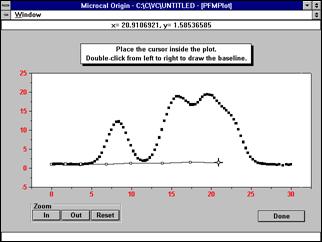
Adjusting the baseline manually
You can manually reshape the baseline by pressing the ![]() button.
This action causes the following window to open:
button.
This action causes the following window to open:
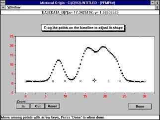
Click on points on the baseline (or on the characteristic baseline basedata_b if the baseline is a regular function) and drag them to new locations to alter the baseline. If the baseline is a function, adjusting its shape is equivalent to adjusting its parameters.
Adding points to a user-drawn baseline
If the selected baseline function is FreeForm or Spline,
points may be added to the baseline from the Phase 2 window without restarting
the fitting session. Press the ![]() button to add more points to the user-drawn
baseline.
button to add more points to the user-drawn
baseline.
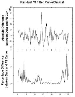
Creating a residual plot
To create a residual plot, press
the ![]() button to open the Peak Results dialog
box. Press the Residual Plot button to
create a residual plot. The residual
plot displays the absolute and percentage difference between the fitted curve
and the original data plot. To return to
the Phase 2 window, press the
button to open the Peak Results dialog
box. Press the Residual Plot button to
create a residual plot. The residual
plot displays the absolute and percentage difference between the fitted curve
and the original data plot. To return to
the Phase 2 window, press the ![]() button.
button.
Fitting a section of data
Fit a section of the data plot by
clicking on the Data Selector tool ![]() in the toolbox in
Origin 4.1 or the Tools toolbar in Origin 5.
Data markers
in the toolbox in
Origin 4.1 or the Tools toolbar in Origin 5.
Data markers ![]() appear at both ends of
the data plot. The range can be adjusted
by moving the two markers on the data plot with the arrow keys, as described in
the status bar. You can also set a range
of data by pressing the
appear at both ends of
the data plot. The range can be adjusted
by moving the two markers on the data plot with the arrow keys, as described in
the status bar. You can also set a range
of data by pressing the ![]() button in the Phase 2 window to open the
Advanced Options dialog box. Press the
Fitting Data Range button to open the Fitting Data Range dialog box. For more information on this dialog box, see
page 36.
button in the Phase 2 window to open the
Advanced Options dialog box. Press the
Fitting Data Range button to open the Fitting Data Range dialog box. For more information on this dialog box, see
page 36.
Setting general linear constraints
General linear constraints are
also supported. Press the ![]() button to open the Advanced Options dialog
box. Press the Linear Constraints button
to open the Set General Linear Constraints dialog box. Enter general linear constraints in this
dialog box. You need to be careful in
using parameter names. If the names are
given as xc, A, w in your function definition, you have to append numbers to
them as they appear in the dialog box, i.e., xc_4, A_4, w_4.
button to open the Advanced Options dialog
box. Press the Linear Constraints button
to open the Set General Linear Constraints dialog box. Enter general linear constraints in this
dialog box. You need to be careful in
using parameter names. If the names are
given as xc, A, w in your function definition, you have to append numbers to
them as they appear in the dialog box, i.e., xc_4, A_4, w_4.
Note: Refer to the Origin User's Manual for more information on linear constraints.
Using weighting in fitting
You can use a weighting method in
the fitting process. Press the ![]() button to open the Advanced Options dialog
box. Press the Weighting Method button
to open the Weighting Method dialog box.
There are four weighting options:
button to open the Advanced Options dialog
box. Press the Weighting Method button
to open the Weighting Method dialog box.
There are four weighting options:
No Weight Used
Instrumental
Statistical
Arbitrary DataSet
If the Arbitrary DataSet option is selected, enter the weighting datasets name (WksName_ColName) in the Weighting DataSet text box.
Reporting results
The PFM can compute various peak characteristics for each peak either interactively or in the form of a report.
To compute peak characteristics interactively:
Press the ![]() button after performing the fit. This action opens the Peak Results dialog
box. Press the Peak Properties button to
open the Peak Characteristics dialog box.
Select the desired peak by pressing either the Prev Peak or Next Peak
buttons. Select the desired peak
characteristic from the Operations drop down list. (If necessary, enter the requested value in
the text box provided.) Press the
Compute button to compute the selected characteristic.
button after performing the fit. This action opens the Peak Results dialog
box. Press the Peak Properties button to
open the Peak Characteristics dialog box.
Select the desired peak by pressing either the Prev Peak or Next Peak
buttons. Select the desired peak
characteristic from the Operations drop down list. (If necessary, enter the requested value in
the text box provided.) Press the
Compute button to compute the selected characteristic.
To generate a report
A Peak
Characterization Report may be generated in the form of a graph, worksheet, or
ASCII file. To generate the report,
press the ![]() button after performing the fit. This action opens the Peak Results dialog
box. Press the Options button
(associated with the desired report format) to open the Peak Characterization
Report Field Details dialog box (for the plot) or the Peak Characterization
Report Details dialog box (for the worksheet).
button after performing the fit. This action opens the Peak Results dialog
box. Press the Options button
(associated with the desired report format) to open the Peak Characterization
Report Field Details dialog box (for the plot) or the Peak Characterization
Report Details dialog box (for the worksheet).
Plot Report (Peak Characterization Report Field Details dialog box):
The default number of report fields is seven. To modify this number, select the desired value from the Total Number of Fields drop down list. Click on 'Peak report field 1' in the Available Fields on Report Plot list box. An associated option is selected in the Available Results for Display list. Modify this selection if desired. Continue this process for each of the 'Peak report field n' fields in the Available Fields on Report Plot list box. Press the OK button after completing the selections.
Press the Plot report format button in the Peak Results dialog box to generate the report.
Worksheet or ASCII File (Peak Characterization Report Details dialog box):
Enable the desired options in the Report Content list box. Press the Return button after completing the selection.
Press the Worksheet or ASCII File report format buttons in the Peak Results dialog box to generate the specified report.
Defining your own function
You can define your own fitting functions. Refer to Chapter 3, 'Fitting Functions', for information on this advanced feature.
Creating a custom initialization file
The PFM can save settings in user-specified initialization files. A particular initialization file may be specified for use at startup, or the PFM may be instructed to read (or write to) an initialization file during operation. In addition, settings saved to a particular initialization file, such as the peak function, number of parameters, and data preconditioning method, are user-defined.
Reading (or Saving to) an Initialization File During a Session:
To view the
settings that may be saved to/or read from a user-specified initialization
file, press the ![]() button to open the Advanced Options dialog
box. Press the Initialization File
button to open the Save/Read Initialization File Options dialog box. Before saving settings to an initialization
file, optimize the desired settings in the current PFM session.
button to open the Advanced Options dialog
box. Press the Initialization File
button to open the Save/Read Initialization File Options dialog box. Before saving settings to an initialization
file, optimize the desired settings in the current PFM session.
To save options to the initialization file listed in the PFM Initialization text box, check the desired options and press the Save button.
To read options from the initialization file listed in the PFM Initialization text box, check the desired options and press the Read button. The current PFM session updates to reflect the specified initialization file settings.
Reading an Initialization File at Startup:
To ensure that the saved parameter values are read when the PFM is launched, press the Parameter Initialization button in the Advanced Options dialog box. This action opens the Parameter Initialization dialog box. Enable the 'Start the PFM using parameters from previous session' check box.
Alternatively, to specify a custom initialization file at startup, enter the desired initialization file in the 'Initialize from' text box in the Phase 0 window.
Very Important Note
Do not use Origin's standard fitting if you are using the PFM module. Conflicts may result.
2 - The PFM Interface
The user-interface of the PFM module is documented in this chapter, including dialog boxes and templates. You can perform your entire peak analysis in this environment.
2.1 Assign Fitting DataSet Dialog Box
To open this dialog
box, press the ![]() button in the Phase 1
window.
button in the Phase 1
window.
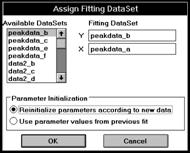
The Available DataSets list box displays all Y datasets in the current project.
The Y and X text boxes display the current Y and X fitting datasets. To replace these datasets, click on the desired Y dataset in the Available DataSets list box. The Assign Fitting Dataset dialog box respects column associations in the worksheet. Thus, the X Fitting DataSet list box automatically updates with the associated X dataset for a given Y Fitting DataSet. This is also the case if the worksheet contains multiple X columns.
Select the 'Reinitialize parameters according to new data' radio button to reinitialize the fitting function parameters according to the currently selected datasets in the Fitting DataSet list boxes. Select the 'Use parameter values from previous fit' radio button to use the parameter values last saved to the initialization file specified in the 'Initialize from' text box in the Phase 0 window.
2.2 Select Fitting Function Dialog Box
To open this dialog
box, press the ![]() button in the Phase 1
window. Additionally, open this dialog
box by clicking on the function name (for the baseline or the desired peak) in
the Phase 2 window.
button in the Phase 1
window. Additionally, open this dialog
box by clicking on the function name (for the baseline or the desired peak) in
the Phase 2 window.
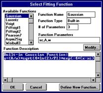
This list box displays the available peak and baseline fitting functions. By default, the following functions are provided:
|
Peak Functions |
|
Baseline Functions |
|
|
Gaussian |
CCE |
NoBase |
ExpDec2 |
|
Gauss2 |
BiGauss |
Constant |
ExpDec3 |
|
EMGauss |
InvsPoly |
Line |
ExpGrow1 |
|
Lorentz |
Sine |
Parabola |
ExpGrow2 |
|
Voigt |
SineSqr |
Cubic |
ExpGrow3 |
|
PsVoigt1 |
SineDamp |
Poly4 |
ExpAssoc |
|
PsVoigt2 |
Power1 |
Poly5 |
Exponent |
|
Pearson7 |
Power2 |
PolyCtr5 |
Hyperbl |
|
Asym2Sig |
Pulse |
Logistic |
DblHypbl |
|
Weibull3 |
DLL_Func |
Boltzman |
Rational |
|
LogNormal |
|
Weibull1 |
Dataset |
|
GCAS |
|
Weibull2 |
FreeForm |
|
ECS |
|
ExpDec1 |
Spline |
All built-in functions are included in this list. Modify the Available Functions list by editing the [FittingFunctions] section of the PFM.INI file.
This list box displays the name of the function selected from the Available Functions drop down list.
This list box displays 'Built-in' or 'User-Script', depending on the function selected from the Available Function drop down list.
This list box displays the total number of parameters for the fitting function selected from the Available Functions drop down list.
This list box displays the parameter names for the function selected from the Available Functions drop down list.
If the function is a built-in function, this text box displays a description of the function. If the function is a user-defined function, this text box displays the definition of the function.
Press this button to open the Modify Peak (or Baseline) Function dialog box. Open this dialog box to modify an existing function. If the function is a built-in function, you cannot modify its function description.
Press this button to open the Define New Peak (or Baseline) Function dialog box. Open this dialog box to create a user-defined function.
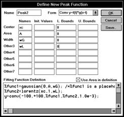
2.2a Modify (or Define New) Function Dialog Box
There are several titles for this dialog box, depending on how it is opened. Edit this dialog box to define a new fitting function or modify an existing one. Open the dialog box by pressing the Modify or Define New Function buttons in the Select Fitting Function dialog box.
This text box lists the default function name. For new functions, default names like Peakn for peaks or Basen for the baselines are suggested. You can modify these names, but avoid using names that are already in use.
There are three forms of user-defined functions available in the Define New Function dialog box: Expression: f(x), Script: y=f(x), and Conv: y=f(t)*g(x-t).
Expression Define your function in an expression format such as:
Y0+A*X+B*X*X
where Y0, A and B are parameters, and X is the independent variable. User-defined functions of this form are fast.
Script Allows you to define functions with multiple lines and intermediate variables such as:
temp1=A*X;
temp2=B*X*X;
Y=temp1+temp2+C;
where temp1 and temp2 are temporary variables. Y is the dependent variable. The great advantage of this form is that you can easily define a large function.
Conv New fitting functions may be defined that are convolutions of built-in PFM functions. For example, to define a function which is a convolution of a Lorentzian and Gaussian function (i.e. a Voigt function), enter the following in the Fitting Function Definition text box:
%func1=gaussian(0,A,wG); /*%func1 is a placeholder.*/
%func2=lorentz(xc,1,wL);
y=conv(-100,+100,%func1,%func2,1.0e-3);
Continue editing the dialog box as follows:
In
this example, gaussian and lorentz are two built-in functions which take three
parameters each. In this instance, the
independent variable is implicit. Please
note that for a function defined as a convolution of two functions, certain
parameters must be given simplifying values.
In this example, the Gaussian peak center is set to zero and the
Lorentzian area to 1. This is to avoid
over-parameterization of the function.
Though '[-100,+100]' was chosen as the x-range for the convolution in
this example, any range could be used up to a maximum range of
[-1.0e-60,1.0e60]. The last argument to
the
conv( ) function (1.0e-3) is the
degree of precision used in evaluating the convolution.
Enter the parameter names in the text boxes provided.
For a peak function, the first three parameters must be prefixed xc (center), A (area or height), and w (width). For a baseline function, the first parameter must be Y0 (offset).
Enter the initial parameter values in the text boxes provided. Use these values to initialize the fitting function.
Enter the lower bounds for the parameters in the text boxes provided. The PFM always presets some bounds for the parameters. For example, the area (A) and width (w) always have greater-than-zero lower bounds.
Enter the upper bounds for the parameters in the text boxes provided.
When checked, the second parameter in the function definition is the area of the peak. When cleared, it is the height of the peak. The default is to use the area.
Enter the definition of the fitting function in this text box.
Press this button to save the current dialog box settings to the function definition file. Additionally, the function is added to the Available Functions drop down list in the Select Fitting Function dialog box.
2.3 Precondition Fitting DataSet Dialog Box
To open this dialog
box, press the button in the Phase 1 window.
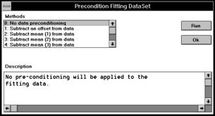
Select the data preconditioning method from this drop down list. Depending on the selected method, associated text boxes display next to the Methods drop down list. For example, if the 'Subtract an offset from data' option is selected, a 'Y offset' text box displays. Enter the desired value in the 'Y offset' text box.
Note:
For reference information on the Tougaard baseline subtraction method,
see
S. Tougaard, Surf. Sci. 216, 343 (1989). For
reference information on the Shirley baseline subtraction method, see D. A.
Shirley, Phys. Rev. B5, 4709
(1972). For a review of both methods,
see S. Tougaard and C. Jansson, Comparison of Validity and Consistency of
Methods for Quantitative XPS Peak Analysis, Surf. Interface Anal. 20, Issue 13, 1013.
This text box provides a description of the selected method from the Methods drop down list.
Press this button to perform the selected preconditioning method.
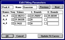
2.4 Edit Fitting Parameters Dialog Box
To open this dialog box, click on the desired fitting parameter in the Phase 2 window. Additionally, this dialog box opens after closing the Select Fitting Function dialog box (in the Phase 2 window).
This list box displays the peak number of the currently displayed peak or baseline. If the number is zero, the function displayed is the baseline.
This list box displays the fitting function name for the currently displayed peak or baseline.
Press this button to display parameter information for the previous peak.
Press this button to display parameter information for the next peak.
The parameter names of the fitting function are listed.
These editable text boxes display the parameter values of the fitting function.
These check boxes allow you to fix parameters to certain values. When checked, the parameter can be modified by the PFM during fitting. Fixing some of the parameters may stabilize fitting. The default status is checked, so the value is varied during fitting. The Vary check box for the first peak function parameter (for each of the peaks) has a direct association with the corresponding peak center control check box in the Phase 2 window. If you enable the Vary check box, the corresponding peak center control check box is enabled (after performing another fit).
These text boxes display the values of the lower bounds for the parameters. Click to enter new values. For some parameters, default bounds are already set. For example, the area of a peak is set to be greater than zero. The default bounds for peak centers are changed dynamically during fitting to keep proper ordering. However, the bounds you enter in this dialog box take precedence.
The check boxes to the left of the L. Bounds text boxes display whether the corresponding parameter bounds are active or disabled. When checked, they are enabled.
These text boxes display the values of the upper bounds for the parameters. Click to enter new values (see above).
If the parameters are modified using this dialog box, pressing this button updates the fit curves in the Phase 2 window.
2.5 Advanced Options Dialog Box
To open this dialog
box, press the ![]() button in the Phase 2 window.
button in the Phase 2 window.
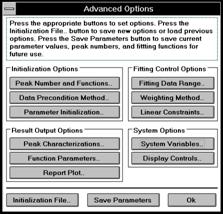
Press the Peak Number and Functions button to open the Peak Number and Functions dialog box.
Press the Data Precondition Method button to open the Select Data Precondition Method dialog box.
Press the Parameter Initialization button to open the Parameter Initialization dialog box.
Press the Peak Characterization button to open the Peak Characterization Report Details dialog box.
Press the Function Parameters button to open the Fitting Function Parameter Report Details dialog box.
Press the Report Plot button to open the Peak Characterization Report Field Details dialog box.
Press the Fitting Data Range button to open the Fitting Data Range dialog box.
Press the Weighting Method button to open the Weighting Method dialog box.
Press the Linear Constraints button to open the Set General Linear Constraints dialog box.
Press the System Variables button to open the System Variables dialog box.
Press the Display Controls button to open the Display Control Options dialog box.
Press the Initialization File button to open the Save/Read Initialization File Options dialog box.
Press the Save Parameters button to open the Save Parameters for Future Use dialog box.
2.5a Fitting Data Range Dialog Box
To open this dialog box, press the Fitting Data Range button in the Advanced Options dialog box.
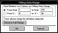
Select a range of data to fit. Row numbers or X values can be used to designate the beginning and ending points of the range. Select the desired radio button and then enter the From and To values in the text boxes provided. For example, select a range from row 20 to row 150 or select all the data from X=13.779 to X=29.854.
Enable the 'Use above range for all future datasets' check box to use the settings in this dialog box for future datasets in the current pfm session.
Press this button to reset to the full data range.
Note: To save these settings for future use, press the Initialization File button in the Advanced Options dialog box. This action opens the Save/Read Initialization File Options dialog box. Enable the 'Fitting Data Range' check box. Press the Save button to save the settings to the specified initialization file. Press the Read button to read the settings from the specified initialization file.
2.5b Weighting Method Dialog Box
To open this dialog box, press the Weighting Method button in the Advanced Options dialog box.
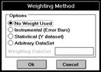
There are four weighting options:
No Weight Used No weight is used.
Instrumental Error bars are used as the weights.
Statistical Square roots of the data points are used as the weights.
Arbitrary DataSet A user-specified dataset is used as the weights.
If the Arbitrary
Dataset option is selected, the name
of the weighting dataset must be entered into the Weighting DataSet text
box. The choice of a
weighting method affects how the sum of squares ![]() , the chi-squares
, the chi-squares![]() and standard errors are calculated.
and standard errors are calculated.
![]() under the four
weighting methods is:
under the four
weighting methods is:
No
Weight Used The sum of
squares is ![]() .
.
Instrumental The plotted error bars are
used as the weights i.e., ![]() .
. ![]() is the error bar size
and is stored in an error bar column.
The sum of squares is
is the error bar size
and is stored in an error bar column.
The sum of squares is ![]() .
.
Statistical The weight is ![]() .
. ![]() is the dependent
variable of the fitting datasets. The
sum of squares is
is the dependent
variable of the fitting datasets. The
sum of squares is ![]() .
.
Arbitrary
DataSet The weight is ![]() .
. ![]() is the data value of
any user-specified column. The sum of
squares is
is the data value of
any user-specified column. The sum of
squares is ![]() .
.
Note: To save these settings for future use, press the Initialization File button in the Advanced Options dialog box. This action opens the Save/Read Initialization File Options dialog box. Enable the 'Weighting Method' check box. Press the Save button to save the settings to the specified initialization file. Press the Read button to read the settings from the specified initialization file.
2.5c Set General Linear Constraints Dialog Box
To open this dialog box, press the Linear Constraints button in the Advanced Options dialog box.
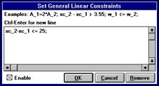
In addition to setting bounds for the parameters, you can set general linear constraints for the parameters. For example, to limit the distance between two peaks to 25, enter xc_2 -xc_1 <= 25 in the dialog box.
When checked, the constraints are enabled. If cleared, the constraints will not affect the parameters.
Press this button to delete the constraints completely.
Note: To save these settings for future use, press the Initialization File button in the Advanced Options dialog box. This action opens the Save/Read Initialization File Options dialog box. Enable the 'Linear Constraints' check box. Press the Save button to save the settings to the specified initialization file. Press the Read button to read the settings from the specified initialization file.
2.5d System Variables Dialog Box
To open this dialog box, press the System Variables button in the Advanced Options dialog box.
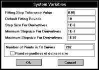
This text box displays the tolerance value
for peak fitting. A smaller value
requires more fitting iterations and should result in more accurate
parameters. The fitting iterations
terminate whenever the relative change of the sum of squares ![]() between successive
iterations is less than the tolerance value.
The relative change of
between successive
iterations is less than the tolerance value.
The relative change of ![]() is defined as
is defined as
 ,
,
where i is the iteration number.
This text box displays the maximum number of
fitting iterations performed after pressing the ![]() button in the Phase 2 window.
button in the Phase 2 window.
This text box value multiplied by the current value of the parameter is used to calculate the step size for the derivative.
If the parameter value becomes too small, such that the parameter multiplied by the step size is less this minimum step size value, then the minimum step size value is used.
If the parameter value becomes too large, such that the parameter multiplied by the step size is greater than this maximum step size value, then the maximum step size value is used.
Enter the number of points used to generate the fit curves in this text box. All curves, e.g., FitFunc_fit, FitFunc_lConf, will have this number of points.
If checked, the number of points specified
in the 'Number of Points in Fit Curves' text box is used for all future fitting
datasets in the current session. If
cleared, the 'Number of Points in Fit Curves' text box value updates when you
load new fitting datasets. (Press the ![]() button in the Phase 1
window to load new fitting datasets.)
button in the Phase 1
window to load new fitting datasets.)
Note: To save these settings for future use, press the Initialization File button in the Advanced Options dialog box. This action opens the Save/Read Initialization File Options dialog box. Enable the 'System Variables' check box. Press the Save button to save the settings to the specified initialization file. Press the Read button to read the settings from the specified initialization file.
2.5e Display Control Options Dialog Box
To open this dialog box, press the Display Controls button in the Advanced Options dialog box.
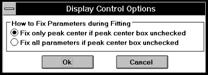
If a peak's peak center check box is cleared in the Phase 2 window:
Select the 'Fix only peak center if peak center box unchecked' radio button to prevent the peak function's peak center parameter from changing during a fit.
Select the 'Fix all parameters if peak center box unchecked' radio button to prevent all the peak function's parameters from changing during a fit.
Note: To save these settings for future use, press the Initialization File button in the Advanced Options dialog box. This action opens the Save/Read Initialization File Options dialog box. Enable the 'Display Controls' check box. Press the Save button to save the settings to the specified initialization file. Press the Read button to read the settings from the specified initialization file.
2.5f Peak Number and Functions Dialog Box
To open this dialog box, press the Peak Number and Functions button in the Advanced Options dialog box.
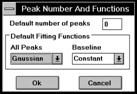
Enter a value for the default number of
peaks in this text box. To display the
individual peak fit curves (or peak function plots), press the ![]() button on the
six-button bar (at the top-right corner of the window).
button on the
six-button bar (at the top-right corner of the window).
Select the default fitting function for all peaks and the baseline from the associated drop down lists.
Note: To save these settings for future use, press the Initialization File button in the Advanced Options dialog box. This action opens the Save/Read Initialization File Options dialog box. Enable the 'Peak Number and Functions' check box. Press the Save button to save the settings to the specified initialization file. Press the Read button to read the settings from the specified initialization file.
2.5g Select Data Precondition Method Dialog Box
To open this dialog box, press the Data Precondition Method button in the Advanced Options dialog box.
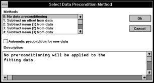
Select the data preconditioning method from this drop down list. Depending on the selected method, associated text boxes display next to the Methods drop down list. For example, if the 'Subtract an offset from data' option is selected, a 'Y offset' text box displays. Enter the desired value in the 'Y offset' text box.
Enable this check box to apply the selected precondition method during data import.
This text box provides a description of the selected method from the Methods drop down list.
Note: To save these settings for future use, press the Initialization File button in the Advanced Options dialog box. This action opens the Save/Read Initialization File Options dialog box. Enable the 'Data Precondition Method' check box. Press the Save button to save the settings to the specified initialization file. Press the Read button to read the settings from the specified initialization file.
2.5h Parameter Initialization Dialog Box
To open this dialog box, press the Parameter Initialization button in the Advanced Options dialog box.
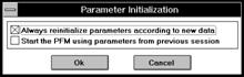
Enable the 'Always reinitialize parameters according to new data' check box to reinitialize the fitting function parameters according to the currently selected datasets in the Assign Fitting DataSet dialog box (Phase 1 window). Enable the 'Start the PFM using parameters from previous session' check box to use the parameter values last saved to the initialization file specified in the Save/Read Initialization File Options dialog box.
Note: To save these settings for future use, press the Initialization File button in the Advanced Options dialog box. This action opens the Save/Read Initialization File Options dialog box. Enable the 'Parameter Initialization' check box. Press the Save button to save the settings to the specified initialization file. Press the Read button to read the settings from the specified initialization file.
2.5i Save/Read Initialization File Options Dialog Box
To open this dialog box, press the Initialization File button in the Advanced Options dialog box.
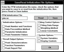
This text box displays the initialization file whose settings may be currently read or set.
When a check box is enabled, the variables may be read to, or set by, the specified initialization file. The variables are set in the following dialog boxes:
Peak Number and Functions, Select Data Precondition Method, and Parameter Initialization. The peak parameter values are displayed in the Phase 2 window.
When a check box is enabled, the variables may be read to, or set by, the specified initialization file. The variables are set in the following dialog boxes:
Peak Characterization Report Details, Fitting Function Parameter Report Details, and Peak Characterization Report Field Details.
When a check box is enabled, the variables may be read to, or set by, the specified initialization file. The variables are set in the following dialog boxes:
Fitting Data Range, Weighting Method, and Set General Linear Constraints.
When a check box is enabled, the variables may be read to, or set by, the specified initialization file. The variables are set in the following dialog boxes:
System Variables and Display Control Options.
Press this button to read the selected variables from the specified initialization file. The variables are applied to the active datasets after closing the Save/Read Initialization File Options and Advanced Options dialog boxes.
Press this button to save the selected variables to the specified initialization file. If the initialization file does not exist, it is created. Otherwise, the specified file is updated.
2.5j Save Parameters for Future Use Dialog Box
To open this dialog box, press the Save Parameters button in the Advanced Options dialog box.
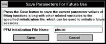
Enter the desired initialization file in this text box. If the initialization file does not exist, it is created. Otherwise, the specified file is updated.
Press this button to save the current parameter values and other related variables (this includes all the variables listed in the Save/Read Initialization File Options dialog box) to the specified initialization file. To use this file to initialize future sessions, enter this initialization file in the 'Initialization from' text box of the Phase 0 window.
2.5k Peak Characterization Report Details Dialog Box
To open this dialog box, press the Peak Characterization button in the Advanced Options dialog box. Alternatively, press the (Worksheet/ASCII File) Options button in the Peak Characterization group of the Peak Results dialog box.
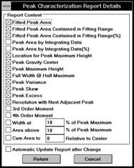
Select the desired report options by enabling the associated check boxes. For clarification on these options, refer to the following definitions:
Fitted Peak Area
Integrate the model function numerically from - to + using the best-fit parameters obtained from the fitting operation.
Fitted Peak Area Contained in Fitting Range
Same as above, but restrict integration to a range that actually has data.
Fitted Peak Area Contained in Fitting Range (%)
Same as above, but expressed as a percent of the total area.
Resolution of two peaks
![]()
where Xc1 and Xc2 are peak centers, w1 and w2 are constructed base widths.
Peak inflection points
The points of inflection are the points of maximum slope on each side of the peak.
Peak moments
![]() (the 0th
moment or the area of the peak)
(the 0th
moment or the area of the peak)
 (the nth
zero-point moment)
(the nth
zero-point moment)
 (the nth
central moment)
(the nth
central moment)
Peak gravity center
![]()
Peak variance
![]()
Peak skew

Peak excess
![]()
Press this button to ensure that the report automatically updates after a change in one of the peak characteristics.
Press this button to complete the selection. To generate the report, press the Worksheet or ASCII File button in the Peak Results dialog box.
Note: To save these settings for future use, press the Initialization File button in the Advanced Options dialog box. This action opens the Save/Read Initialization File Options dialog box. Enable the 'Peak Characterizations' check box. Press the Save button to save the settings to the specified initialization file. Press the Read button to read the settings from the specified initialization file.
2.5l Fitting Function Parameter Report Details Dialog Box
To open this dialog box, press the Function Parameters button in the Advanced Options dialog box. Alternatively, press the (Worksheet/ASCII File) Options button in the Fitting Function Parameters group of the Peak Results dialog box.
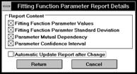
Enable the desired parameter report options in this group. The selected options are used to create/update the Param worksheet values (associated Worksheet button in the Peak Results dialog box) or the ASCII file values (associated ASCII File button in the Peak Results dialog box).
Enable this check box to automatically update the Param worksheet if the parameters change after a fit.
Press this button to save the settings and return to the Peak Results dialog box.
Note: To save these settings for future use, press the Initialization File button in the Advanced Options dialog box. This action opens the Save/Read Initialization File Options dialog box. Enable the 'Function Parameters' check box. Press the Save button to save the settings to the specified initialization file. Press the Read button to read the settings from the specified initialization file.
2.5m Peak Characterization Report Field Details Dialog Box
To open this dialog box, press the Report Plot button in the Advanced Options dialog box. Alternatively, press the (Plot) Options button in the Peak Characterization Report group of the Peak Results dialog box.
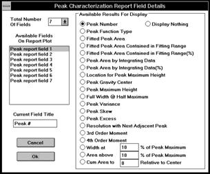
Select the desired number of report fields from this drop down list.
Select the currently active field from this list box. Note that the currently selected result option becomes activated in the Available Results For Display group. Additionally, the associated default title displays in the Current Field Title text box.
This text box displays the default title for the report option associated with the active field. Modify this title as desired.
Select the desired report option (for the active field) by clicking on the associated radio button. For information on these options, see page 49.
Note: To save these settings for future use, press the Initialization File button in the Advanced Options dialog box. This action opens the Save/Read Initialization File Options dialog box. Enable the 'Peak Report Plot' check box. Press the Save button to save the settings to the specified initialization file. Press the Read button to read the settings from the specified initialization file.
2.6 Peak Results Dialog Box
To open this dialog
box, press the ![]() button in the Phase 2 window.
button in the Phase 2 window.
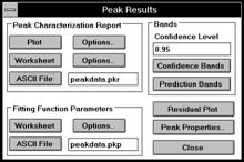
Press the Plot button to generate the Report graph window which contains data plots of the original data and the fit curves, together with the peak parameters specified in the Peak Characterization Report Field Details dialog box (accessed from the associated Options button). This window is based on the PKREPORT.OTP template, which can be modified according to your needs as described in the graph window.
Press the Worksheet button to generate the ReportWks worksheet window which contains the peak parameter values specified in the Peak Characterization Report Details dialog box (accessed from the associated Options button).
Press the ASCII File button to create the specified ASCII file which contains the peak parameter values specified in the Peak Characterization Report Details dialog box (accessed from the associated Options button).
Press the Worksheet button to generate the Param worksheet which contains the fitting function parameter properties specified in the Fitting Function Parameter Report Details dialog box (accessed from the associated Options button). See the Param Worksheet section for details.
Enter the desired confidence level in the associated text box.
Press the Confidence Bands button to generate confidence bands for the fit curve.
Press the Prediction Bands button to generate prediction bands for the fit curve.
Press this button to create a residual
plot. The residual plot displays the
absolute and percentage difference between the fit curve and the original data
plot. To return to the Phase 2 window,
press the ![]() button.
button.
Press this button to open the Peak Characteristics dialog box (see the following section).
2.6a Peak Characteristics Dialog Box
To open this dialog box, press the Peak Properties button in the Peak Results dialog box. Use this dialog box to compute results interactively.
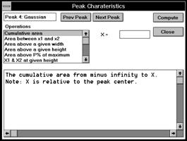
Press this button to return to the previous peak.
Press this button to advance to the next peak.
Select the desired peak characteristic from this drop down list.
If displayed, enter the requested value in this text box. (This text box is not displayed for all selections from the Operations drop down list.)
Press this button to compute the selected characteristic.
2.6b Param Worksheet
|
Function |
ParaName |
Value |
Error |
ConfIntvl |
Depend |
|
Constant |
Y0 |
0.99367 |
0.01801 |
0.0353 |
0.68042 |
|
Gaussian |
xc_1 |
8.29528 |
0.0059 |
0.01157 |
0.00552 |
|
|
A_1 |
35.43495 |
0.18521 |
0.36301 |
0.59416 |
|
|
w_1 |
2.94465 |
0.01522 |
0.02984 |
0.44698 |
|
Gaussian |
xc_2 |
15.46965 |
0.03025 |
0.05929 |
0.97806 |
|
|
A_2 |
61.88892 |
1.50592 |
2.9154 |
0.99258 |
|
|
w_2 |
3.55953 |
0.03584 |
0.07025 |
0.94223 |
|
Gaussian |
xc_3 |
19.67063 |
0.02677 |
0.05246 |
0.97121 |
|
|
A_3 |
83.76968 |
3.38002 |
6.62471 |
0.99818 |
|
|
w_3 |
4.39459 |
0.1566 |
0.30693 |
0.99689 |
|
Gaussian |
xc_4 |
22.85883 |
0.0435 |
0.08527 |
0.96156 |
|
|
A_4 |
22.07233 |
2.04396 |
4.00608 |
0.99689 |
|
|
w_4 |
2.74944 |
0.07003 |
0.13726 |
0.94517 |
|
SS |
|
0.92124 |
|
|
|
|
ChiSqr |
|
0.01047 |
|
|
|
|
COD |
|
0.99981 |
|
|
|
|
Correlation |
|
0.9999 |
|
|
|
|
DOF |
|
88 |
|
|
|
|
NPoints |
|
101 |
|
|
|
|
Confidence |
|
0.95 |
|
|
|
|
Tolerance |
|
0.05 |
|
|
|
The upper part of the worksheet displays information on the fitting functions and related parameters. The parameter names, values, errors, confidence interval, and dependency are given.
The lower half of the worksheet displays the following variable values:
SS: Sum of squares.
ChiSqr: Chi-square value.
COD: Coefficient of determination.
Correlation: Correlation coefficient.
DOF: Degree of freedom.
NPoints: Number of data points used in the fitting.
Confidence: Confidence level used in calculating confidence limits, confidence and prediction bands.
Tolerance: Tolerance value used in fitting.
For more information on these variables, see the Origin User's Manual.
2.6c Report Graph Window
Generate a fitting report graph by pressing the ![]() button in the Phase 2 window. This action opens the Peak Results dialog box. Press the Plot
button in the Peak Characterization Report group to create a graph window named
Report. The Report graph contains the results specified in the Peak Characterization Report Field Details dialog box (opened from the
(Plot) Options button in the Peak Characterization Report group). The contents are described below.
button in the Phase 2 window. This action opens the Peak Results dialog box. Press the Plot
button in the Peak Characterization Report group to create a graph window named
Report. The Report graph contains the results specified in the Peak Characterization Report Field Details dialog box (opened from the
(Plot) Options button in the Peak Characterization Report group). The contents are described below.
Source File The data source file, usually is the name of the worksheet that contains the fitting data.
Dataset The Y fitting dataset name.
Date The date the report is generated.
Chi^2= The Chi-Square value.
COD= The coefficient of determination value.
# of Data Points= The number of data points used in the fitting.
SS= The sum of squares.
Corr Coef= The correlation coefficient.
Degree of Freedom= The degree of freedom.
The graph includes the original data plot (displayed with small black squares), the fitted curve, all peak curves, and the baseline curve.
This section includes the descriptive results for the peaks. The fields are determined by the settings in the Peak Characterization Report Field Details dialog box (press the (Plot) Options button in the Peak Results dialog box). For a discussion of these fields, see page 49.
The baseline function displays at the bottom of the Report graph window.
2.6d ReportWks Worksheet
Generate a fitting
report worksheet by pressing the ![]() button in the Phase 2 window. This action opens the Peak Results dialog box. Press the
Worksheet button in the Peak Characterization Report group to create a
worksheet window named ReportWks. The
ReportWks worksheet contains the
results specified in the Peak Characterization Report Details dialog box (opened from the (Worksheet) Options button in
the Peak Characterization Report group).
For a discussion of these fields, see page 49.
button in the Phase 2 window. This action opens the Peak Results dialog box. Press the
Worksheet button in the Peak Characterization Report group to create a
worksheet window named ReportWks. The
ReportWks worksheet contains the
results specified in the Peak Characterization Report Details dialog box (opened from the (Worksheet) Options button in
the Peak Characterization Report group).
For a discussion of these fields, see page 49.
|
PeakNum |
PeakType |
Center |
AreaFit |
AreaData |
Height |
Width |
WidHM |
|
1 |
Gaussian |
99.64 |
46318.90 |
46311.8255 |
63827.51 |
0.4834 |
0.48345 |
|
2 |
Gaussian |
100.62 |
74776.93 |
74773.7649 |
82359.04 |
0.4890 |
0.48908 |
|
3 |
Gaussian |
101.61 |
9581.97 |
9581.1632 |
53361.45 |
0.4941 |
0.4941 |
|
4 |
Gaussian |
102.75 |
8723.15 |
8723.04068 |
13650.44 |
0.5276 |
0.52768 |
2.7 PkPhase1.otp Template
The Phase 1 window opens after pressing the ![]() button in the Phase 0
window. Use this window to select
fitting datasets and fitting functions, precondition the data, integrate the
peak areas, and perform initial parameter estimations.
button in the Phase 0
window. Use this window to select
fitting datasets and fitting functions, precondition the data, integrate the
peak areas, and perform initial parameter estimations.
Because the data selected from the worksheet is already loaded when this window opens, you will rarely use this button. However, if you want to change the fitting dataset after the Phase 1 window is opened, press this button to open the Assign Fitting DataSet dialog box. For more information on this dialog box, see page 25.
The peak function defaults to the function specified in the
initialization file read at start-up.
Change the default function for all of the peaks by pressing this button
to open the Select Fitting Function dialog box. For more information on this dialog box, see
page 26. (If you want to assign a different function
for each peak, press the ![]() button to open the
Phase 2 window.)
button to open the
Phase 2 window.)
The baseline function defaults to the function specified in the initialization file read at start-up. Change the default function by pressing this button to open the Select Fitting Function dialog box. For more information on this dialog box, see page 26. To draw a line to be used as the baseline, select FreeForm or Spline from the Available Functions list box.
After pressing this button, the window appears as shown below. Double-clicking at locations which are roughly the peak center-tops provides an estimation of the peaks center and height. This information is used for the initial parameter values during the fitting.
Peak
center-top locations. Double-click at these locations to set the peak
center and height![]()
![]()
![]()
![]()
![]()
![]()
![]()
![]()
Press this button to precondition the data prior to fitting. This action opens the Precondition Fitting DataSet dialog box. For more information on this dialog box, see page 31.
Press this button to find the area of your peaks by numerical integration of the data (via the trapezoidal rule). For more information on this option, see page 13.
Press this button to reinitialize the PFM and discard all parameters.
Press this button to open the Phase 2 window.
2.8 PkPhase2.otp Template
The Phase 2 window opens after pressing the ![]() button in the Phase 1
window.
button in the Phase 1
window.
![]()
![]()
![]()
![]()
![]()
![]()
![]()
![]()
![]()
![]()
![]()
![]()
![]()
![]()
![]()
![]()
![]()
![]()
![]()
![]()
![]()
![]()
![]()
![]()
![]()
![]()
![]()
![]()
1. Opens the Select Fitting Function dialog box. Select a fitting function or define a new one for the peak.
2. Opens the Edit Fitting Parameters dialog box. Edit fitting parameters for the peak.
3. Toggles between creating peak function plots for all peaks and removing them.
4. Toggles between overlaying the peak function plots on the baseline and removing the baseline from all peak function plots.
5. Sets a fitting function for all peaks. Pressing this button is the same as pressing the Set Peak Function button in the Phase 1 window.
6. Sets a baseline function. This is the same as the Set Baseline button in the Phase 1 window.
7. Add new peaks to the function plot. This is the same as the Estimate Peaks' Center and Height button in the Phase 1 window.
8. Delete the highlighted peak.
9. Toggles between creating and removing a peak function plot for the pointed peak.
10. Toggles between overlaying and removing a peak function plot on the baseline.
11. Scrolls among peaks.
12. Peak-width general object. If checked, all peaks have the same width.
13. Peak-width object. If checked, the peak below will have the same width as other checked peaks.
14. Peak-center general object. If checked, all peak centers can vary during fitting iterations.
15. Peak-center object. If checked, the center of the peak below can vary during fitting iterations.
16. If cleared, the parameters of the baseline are not changed during fitting iterations.
17. The peak-center lines can be dragged to adjust peak locations.
18. The height-line can be dragged to move the baseline up and down (adjusting the offset Y0).
19. Adjust the baseline shape by pressing this button.
20. Subtract the baseline from the original fitting data or add it back.
21. Press this button to add more points to a user-drawn baseline.
22. The original dataset displays with black squares.
23. The fit function curve FitFunc_fit displays as a red line.
24. The fit function curve for peak n (FitFunc_fn) displays as a blue line.
25. If the baseline is a hand-drawn line, these red dots are the hand-drawn line basedata_b. Otherwise, it is the characteristic points of the baseline function, with the number of points equal to the number of parameters of the baseline function. We call basedata_b the characteristic baseline. You can manually adjust the shape of the baseline by pressing button 19.
In principle, the parameter values of a function with n parameters can be determined given n pairs of X-Y values. This can be done exactly for functions like the Parabola function, while for functions like the Boltzman function the parameters can only be determined approximately in a least-squares sense. The basedata_b dataset is used to determine the parameters of the baseline. Adjusting its shape is equivalent to adjusting the parameters of the baseline function.
26. Chi-Square value. Its definition is
![]() ,
,
![]() is the sum of squares
value defined below, p is the parameter vector, d is
the degree of freedom, n is the
number of data points used in computation, and p is the number of varying parameters in fitting.
is the sum of squares
value defined below, p is the parameter vector, d is
the degree of freedom, n is the
number of data points used in computation, and p is the number of varying parameters in fitting.
27. Sum of squares value. Its definition is
![]() ,
,
![]() is the function value
evaluated for data point i,
is the function value
evaluated for data point i, ![]() is the weight, and i is incremented by
is the weight, and i is incremented by ![]() . The PFM actually
implements the Levenberg-Marquardt algorithm to find the parameters p to minimize
. The PFM actually
implements the Levenberg-Marquardt algorithm to find the parameters p to minimize ![]() . The weight
. The weight ![]() specifies the contribution
from data point i. There are four types of weighting methods
which are described on page 37.
specifies the contribution
from data point i. There are four types of weighting methods
which are described on page 37.
28. Correlation coefficient.
Fits for up to 10 iterations or fits up to the number specified in the Default Fitting Rounds text box of the System Variables dialog box (System Variables button in the Advanced Options dialog box).
Opens the Peak Results dialog box.
Opens the Advanced Options dialog box.
Resets to the Phase 1 window. Nothing is changed. However, you can load new datasets.
2.9 Reserved Variables, Datasets, Objects, and Macros
Some variables, datasets, and objects are reserved for the PFM interface and are listed below. Items with an n at the end stand for a number of similar names, i.e., clinen means that there is a list of variables: cline0, cline1, cline2, etc. You should not delete these variables, datasets, or objects, nor should you create other variables, datasets, or objects with the same names.
PeakCur Used in building templates.
NoUpdate Used in building templates.
BaseData_A The x column of the baseline.
BaseData_B The y column of the baseline.
FitFunc_xVal The x column of the function plots.
FitFunc_fit The fit curve.
FitFunc_fn The fit curve of a single peak function.
BaseLine_a The x column of the internal baseline.
BaseLine The y column of the internal baseline.
Objects in the pkPhase2.otp template
|
bBase |
parascrl |
pkparan |
WCBOXn |
|
CLINEn |
peakfile |
pkSetPara |
wcLine |
|
doSel |
pkChiSqr |
rescale |
WinClose |
|
Fitcontrol |
pkFuncAll |
rescale2 |
WinOpen |
|
msgdisp |
pkparaline |
WCBOX |
|
Objects in the pkPhase1.otp template
|
bsfdisp |
loadData |
rescale2 |
SetPkfunc |
|
CLINEn |
peakfile |
Restart |
Startsessn |
|
datadisp |
pkfdisp |
SetBsfunc |
WinClose |
|
doSel |
rescale |
setpeakxc |
WinOpen |
Objects in the pkPhase3.otp, pkPhase4.otp and pkPhase5.otp templates
|
doSel |
rescale |
Stopbutn |
WinOpen |
|
MsgDisp |
rescale2 |
WinClose |
Zoom |
|
peakfile |
|
|
|
Objects in the pkReport.otp template
|
rPkArea |
rPkData |
rPkHeight |
rPkType |
|
rPkBase |
rPkFile |
rPkNum |
XTitle |
|
rPkCenter |
rPkFWHM |
rPkPercen |
YTitle |
For a listing, including definitions, of the macros used by the PFM, view EASYPEAK.CNF located in the Origin directory.
3 - Fitting Functions
The PFM module allows users to fit their data to any function. Most common models are built-in functions which offer exceptional speed and reliability. You may also choose your own functional form through user-defined functions. In this chapter, all of the built-in functions are documented, and the use of user-defined functions is explained in detail.
3.1 Conventions For Fitting Functions
There are three types of built-in functions: peak-shaped, non-peak-shaped, and periodic. The peak-shaped and periodic functions are used as peak functions, and the non-peak-shaped functions are used as baseline functions. However, you can also use a peak-shaped function as the baseline function. For example, you can use a Gaussian tail as the baseline. See section 3.8, Advanced Features, for information on using peak-shaped functions as the baseline.
The PFM allows you to define your own functions. There are certain conventions to follow when doing so. First, do not use function names that have already been used by other functions. Second, do not use reserved system variables as parameter names. The first parameter of a peak function should be the center of the peak (xc), the second should be the area or amplitude of peak (A), and the third be the width of the peak (w). Similarly, the first parameter of a baseline function should be the offset (Y0). These conventions can only be circumvented by using scripts to develop your own application.
The parameter names of a fitting function have a specific meaning. A typical example is that w is used for the width of a peak. Whenever there are two or more peaks with the same function or there are parameters with the same name, the parameters are post-appended with numbers, such as w_1 and w_2. These parameters are assumed to have different values in general. Thus, if the widths of some peaks are inherently equal, you will have to set them by checking the width object check boxes in the Phase 2 window.
Each function has an associated function definition file with extension *.PKF in the FITFUNC directory. These files are loaded in when the PFM performs its initialization procedure. You can modify these files to change their properties. See section 3.7 for an explanation of the *.PKF files.
3.2 Built-in Peak Functions
![]()
xc: Center
A: Peak area
w: Full width at half maximum
Gaussian function in the form used for chromatography:
![]()
![]() : Time of peak
max; the retention time
: Time of peak
max; the retention time
A: Peak area
Exponentially modified Gaussian function
![]()
The Lorentzian function:
xc: Center
A: Peak area
w: Full width at half maximum
A: Peak area
xc: Center
wG : Full Gaussian width at half maximum
wL : Full Lorentzian width at half maximum
![]() is called the damping
constant. This function is very slow to
compute due to the infinite integral.
is called the damping
constant. This function is very slow to
compute due to the infinite integral.
Pseudo-Voigt function, type 1:
A: Amplitude
xc: Center
w: Full width at half maximum
mu: Profile shape factor
Gaussian and Lorentzian have the same width.
Pseudo-Voigt function, type 2:
A: Amplitude
xc: Center
wG : Full Gaussian width at half maximum
wL : Full Lorentzian width at half maximum
mu: Profile shape factor
Gaussian and Lorentzian can have different widths.
PearsonVII function:
A: Area
xc: Center
w: Full width at half maximum
m: Profile shape factor
Asymmetric double sigmoidal function:
A: Amplitude
xc: Center
w1 : Width 1
w2 : Width 2
w3 : Width 3
A: Amplitude
xc: Center
w1 : Width 1
w2 : Width 2
![]()
Xc, H, and w are function parameters.
Gram-Charlier A-Series
![]()
![]()
rt : Time of peak max; the retention time
A: Peak area
![]() : Standard
deviation of the peak
: Standard
deviation of the peak
A3 : Skew
A4 : Excess
H3 : z3-3z
H4 : z4-6z3+3
Edgeworth-Cramer Series
![]()
![]()
rt : Time of peak max; the retention time
A: Peak area
![]() : Standard
deviation of the peak
: Standard
deviation of the peak
A3 : Skew
A4 : Excess
H3 : z3-3z
H4 : z4-6z3+3
H6 : z6-15z4+45z2-15
Chesler-Cram equation
![]()
C1 : Peak height
C4 : Time of peak max; the retention time
Asymmetrical Gaussian function
rt :: Time of peak max; the retention time
xc : Peak center
H : Peak height
![]() : Left standard
deviation of the peak
: Left standard
deviation of the peak
![]() : Right standard
deviation of the peak
: Right standard
deviation of the peak
Inverse polynomial function:
A: Amplitude
xc: Center
w: Width
A1: Coefficient
A2: Coefficient
A3: Coefficient
When A1 = 1, A2 = 0, A3 =
0, this function is Lorentzian. When
A1
= 1, A2 = 1/2, A3 = 1/6, this
function approximates a Gaussian.
See page 86.
See page 86.
See page 86.
![]()
xc: Center
A: Amplitude
p: exponent
![]()
xc: Center
A: Amplitude
p1: Left exponent
p2: Right exponent
A: Amplitude
3.3 Baseline Built-in Functions
This is a special function which allows for no baseline.
y = Y0
![]()
A: Intercept
B: Slope
![]()
![]()
![]()
![]()
Built-in 5th order centered polynomial function.
![]()
![]()
xc: Center
![]()
Y0: Offset
A1: Initial value
A2: Final value
xc: Center
p: Power
![]()
The Boltzman function:
Y0: Offset
A1: Initial value
A2: Final value
xc Center
w: width
![]()
Y0: Offset
xc: Center
A: Amplitude
r0: Rate
mu: Exponent
![]()
Y0: Offset
A1: Initial value
A2: Final value
r0: Rate
mu: Exponent
![]()
![]()
![]()
![]()
![]()
![]()
A double exponential association function.
![]()
The exponential function:
Y0: Offset
A: Initial value
R0: Rate
![]()
A rectangular hyperbola function.
![]()
A double rectangular hyperbola function.
![]()
See page 87.
See page 87.
See page 87.
3.4 Periodic Built-in Functions
The fitting functions in this section are periodic functions. They are used in the same way as the peak functions with two exceptions. First, these functions will apply to all peaks when selected. Second, automatic initialization cannot be performed, so you must initialize the function parameters.
![]()
A: Amplitude
xc: Center
w: Width
t0: Decay time
![]()
A: Amplitude
xc: Center
w: Width
![]()
A: Amplitude
xc: Center
w: Width
3.5 Special Functions Dataset, FreeForm and Spline
There are three special baseline functions: Dataset, FreeForm, and Spline.
A user-drawn line with points connected by straight line segments is used as the baseline. After you have selected this function from the Select Fitting Function dialog box, a new window displays. Double-click to draw the line. Internally, a dataset named baseLine is created and used for the actual computation.
A user-drawn line with points connected by cubic spline segments is used as the baseline. After you have selected this function from the Select Fitting Function dialog box, a new window displays. Double-click to draw the line. Internally, a dataset named baseLine is created and used for actual computation.
A dataset is used as the baseline. After you have selected this function from the Select Fitting Function dialog box, you are prompted to enter the dataset name. The dataset name should be in the form WorksheetName_ColName. For example, Data2_B specifies the B column dataset within the worksheet Data2. Internally, a dataset named baseLine is created and used for the actual computation.
3.6 User-supplied Functions
The advantage of built-in functions is their speed. If none of the built-in functions fit to your data, you will need to define your own functions. The PFM module allows you to define new functions. There are certain restrictions on defining new functions. Specifically, you have to follow the format of a user-defined function. Additionally, do not use any system variables as parameters. To view the system variables, type list v in the Script window (Window:Script Window).
First, refer to the PFM Interface chapter for information on opening the Select Fitting Function dialog box. Press the Define New Function button. This action opens the Define New Peak/Baseline Function dialog box.
In this example, a baseline function of a parabola form is defined:
![]()
Pressing the Define New Function button in the Select Fitting Function dialog box opens the Define New Baseline Function dialog box as shown below:
The first parameter is already prefixed to Y0. Form defaults to Expression: f(x). The function name defaults to Base1. Follow the steps below:
Step 1 Enter the other two parameters as A and B.
Step 2 Select Form Expression: f(x). (For more information on available forms, see page 28.)
Step 3 Move the cursor into the Fitting Function Definition text box and type in your own function as:
Y0+A*X+B*X*X
Step 4 You can change the function name to any name with less than 8 characters, as long as it is unique to this function.
Step 5 Press the Save button to save the function for future use.
Step 6 Press the OK button.
In this example, we define a peak function which is a modified version of the Gaussian function:
This function is more complicated than the baseline function in the previous example. Select Script y=f(x) from the Form drop down list so that we can define a multiple-line script function. Type in the function definition shown below into the Fitting Function Definition text box:
temp1=(X-XC)/W;
temp2=temp1*temp1;
Y=A*exp(-2*(temp2+B*temp2*temp2))/(W*sqrt(PI/2));
Here temp1 and temp2 are two temporary variables. The first three parameters are already defaulted to xc, A, and w. You only need to enter the fourth parameter B. In addition, give B an initial value of 0.05 and a lower bound to guarantee that it is always greater than zero. Make sure that the 'Use Area in definition' check box is checked since A is the area in this definition. The dialog box should appear as follows:
New fitting functions may be defined that are convolutions of built-in PFM functions. Fitting functions defined as convolutions will be somewhat slower than script, built-in or DLL functions, and should be used with care. For an example of a convolution of a Lorentzian and a Gaussian function (i.e. a Voigt function), see page 29.
External DLLs may be used as fitting functions for peaks or baselines. This procedure is nearly identical to the process for using external DLLs as regular Origin fitting functions, detailed in the Origin Professional Manual (also available from Microcal Software, Inc.).
A sample fitting function DLL (DLL_FUNC.DLL) is included with the PFM, along with its source code (DLL_FUNC.C), module definition file (DLL_FUNC.DEF), and its required header file (LABFIT.H). Also included is a function definition file (DLL_FUNC.PKF) for the one function which the DLL contains, a simple Gaussian function.
The following steps illustrate the use of this function in the PFM. Note that this Gaussian DLL function is already installed for you, but the steps are included here by way of example.
1. Copy the DLL into the Origin software directory where the Origin executable file and the PFM DLL are installed.
2. Copy the function definition file DLL_FUNC.PKF into the FITFUNC subdirectory.
3. Edit the PFM.INI file so that the PKF file name (in this case DLL_FUNC) appears in the appropriate list (PeakFuncList or BaseFuncList) in the [FittingFunctions] section of PFM.INI.
After completion of these steps and re-starting the PFM, the function appears in the associated function drop down list of the Peak Number and Functions dialog box. Note that the name of the DLL, the name of the function in the DLL, and the name of the PKF file are distinct though they are all DLL_FUNC in this example. That is to say:
The DLL name is user-defined. A single DLL may contain many functions.
The name of the function(s) in the DLL are the actual C identifiers used in the source code to prototype and define the function. This function name must appear in the EXPORTS section of the module definition (DEF) file with an ordinal number which is used to refer to the function.
The function definition file (PKF file) must contain the name of the DLL and the ordinal number of the appropriate function in the NAME field.
The name of the function definition file (PKF file, not the DEF file) is the name that will appear in the drop down list for peak or baseline functions. It is distinct from the DLL name, or the names of any functions exported in the DLL.
The source code for the sample DLL is commented and can be modified to provide any function desired.
The function definition file for a DLL function can be modified from the sample DLL_FUNC.PKF provided, but must comply with the following requirements:
The fields NPARAM and PARAMETERS should be edited so the number of parameters and their names match what is required by the DLL.
The parameters must always be in the order center, area, width, (others) for a peak function and offset, (others) for a baseline function.
Initial values for parameters may be edited in the INITVAL field. To leave any parameter to be set by the user, place a # in that parameters position.
UPPERBOUND and LOWERBOUND fields may also be edited with some restrictions. Area and width parameters must have a lower bound of 0 and center parameters should be left with a !. This instructs the PFM to determine the bounds for that parameter. In addition, the parameters may vary during the fitting session.
The last element in the OPTIONS field should be set to the keyword PEAK or BASE, depending on which type of function you intend.
All other fields in the PKF file should be left as they are, except for FORMULA, which may be updated. In the case of DLL functions, the FORMULA field is merely a description of the function for the users benefit. For user-defined script functions, this field actually defines the function and must therefore follow proper LabTalk syntax.
3.7 Functions Accessible from LabTalk
Any built-in function, user-defined script function, function defined as a convolution of two built-in functions, or external DLL function may be invoked from LabTalk using the syntax pf.f_funcname(x-value,parameters). Funcname is the name of the function, x-value is the value at which you desire the function to be evaluated (or the variable 'x', in the case of function plots), and parameters is a list of parameters (given either as literal values or via LabTalk variables) appropriate to the function. Invoking built-in functions in this manner is much quicker than the equivalent user-defined function.
New functions can be created using this method. For example, you can define a user-defined function: pseudo-Voigt function in Expression form (as selected from the drop down list).
mu*pf.f_gaussian(x, xc, A, wG) + (1-mu)*pf.f_lorentz(x, xc, A, wL)
Please note that these functions are only accessible in this way when the PFM DLL is loaded as the LabTalk command object pf, and the module has been properly initialized.
3.7 Function Definition Files
Every built-in and user-defined function has an associated function definition file stored in the FITFUNC subdirectory. These files have the file extension .PKF. They are created and altered automatically by the PFM when you make changes to the Modify Fitting Function dialog box. Only users who are interested in developing their own peak fitting applications will need to access these files directly. A function definition file has the form:
NAME=Gaussian
NPARAM=3
PARAMETERS=xc,A,w
MEANINGS=center, area, width
INITVAL=#,#,#
LOWERBOUND=#,0,0
UPPERBOUND=#,#,#
FORMULA=
OPTIONS=BUILTIN,CAL,FIT,WIDTH,DERIV,PEAK
Each item in the file is defined in this section.
The name of the fitting function if the function is user-defined, i.e., it is the same as the name of the function definition file. If the function is a built-in function, it is the name of the internal function, and the function definition file can have a different name.
The number of parameters.
The parameter list. These parameter names are appended with numbers to avoid duplicate names. For example, A_1 for peak 1 and A_2 for peak 2.
The initial parameter values. Their order must be the same as the parameters. # is used to denote that there is no initial value for the corresponding parameter.
The lower bounds of parameters. Their order must be the same as the parameters. # is used to denote that there is no lower bound for the corresponding parameter.
The upper bounds of parameters. Their order must be the same as the parameters. # is used to denote that there is no upper bound for the corresponding parameter.
The definition of the function if the function is user-defined, or the description if it is built-in.
The properties of the function, which typically determine how to initialize the function. They are listed as follows:
BUILTIN Built-in function.
USERSCRIPT User-defined function.
EXPRESSION User-defined function of the expression form.
YSCRIPT User-defined function of the y-script form.
CAL Can be initialized by calculation (only applies to built-in functions).
FIT Can be initialized by test-fitting (a half-featured fit).
HEIGHT Parameter A (the second parameter) is the peak height rather than the area. Without this option, parameter A is the area. (This option is typically used for peak functions.)
UP Increasing function. This option is typically used for baseline functions.
DOWN Decreasing function. This option is typically used for baseline functions.
WIDTH Parameter w is exactly the full width at half maximum height of the peak. This option is typically used for peak functions.
DERIV Derivatives of the function are calculated internally. This option only applies to the built-in functions.
PEAK Peak function.
BASE Baseline function.
PERIODIC Periodic function.
EXPLICIT No way to initialize parameters internally, so users must provide initial parameter values.
3.8 Advanced Features
The functions in the Available Functions list box of the Select Fitting Function dialog box are determined by the initialization file PFM.INI. There is a section [FittingFunctions] in the PFM.INI:
[FittingFunctions]
path=fitfunc
PeakFuncList = Gaussian Gauss2 EMGauss Lorentz Voigt PsVoigt1 PsVoigt2 Pearson7 Asym2Sig Weibull3 LogNorml GCAS ECS CCE BiGauss InvsPoly Sine SineSqr SineDamp Power1 Power2 Pulse Dll_Func Peak4
BaseFuncList = NoBase Constant Line Parabola Cubic Poly4 Poly5 PolyCtr5 Logistic Boltzman Weibull1 Weibull2 ExpDec1 ExpDec2 ExpDec3 ExpGrow1 ExpGrow2 ExpGrow3 ExpAssoc Exponent Hyperbl DblHypbl Rational DataSet FreeForm Spline
PeakFuncList and BaseFuncList list the visible functions in the Select Fitting Function dialog box. By default, all built-in functions are listed. You can modify the initialization file to include or exclude functions. Path is the subdirectory for fitting functions.
You can use a peak-shaped function as the baseline function. This is done by creating a new function definition file, and adding the peak function name into the BaseFuncList in the PFM.INI file. The following example uses a Gaussian function as the baseline to demonstrate the basic idea. The Gaussian function used as the baseline has the form Gaussian(Y0, xc, A, w):
![]()
rather than Gaussian(xc, A, w)
![]()
A new function definition file is needed.
Step 1: Make a copy of the function definition file of the Gaussian function (usually located in the FITFUNC subdirectory). Give it a new name: GAUSSBAS.PKF.
Step 2: Edit the new function definition file GAUSSBAS.PKF in any text editor such as NotePad. Modify the file as follows. Changes are marked in bold, italicized text. Note the name is still Gaussian because the built-in function is still used for computation. The function name will appear as GaussBas in the Available Functions list.
|
File Gaussian.pkf |
|
File GaussBas.pkf |
|
NAME=Gaussian |
|
NAME=Gaussian |
|
NPARAM=3 |
|
NPARAM=4 |
|
PARAMETERS=xc,A,w |
|
PARAMETERS=Y0,xc,A,w |
|
INITVAL=#,#,# |
|
INITVAL=#,#,#,# |
|
LOWERBOUND=#,0,0 |
|
LOWERBOUND=#,#,0,0 |
|
UPPERBOUND=#,#,# |
|
UPPERBOUND=#,#,#,# |
|
FORMULA= |
|
} |
|
OPTIONS=BUILTIN,CAL,FIT,WIDTH,DERIV,PEAK |
|
OPTIONS=BUILTIN,CAL,FIT,WIDTH,DERIV, PEAK,BASE |
Step 3: Edit the PFM.INI file to include the new function GaussBas. Put the function into the BaseFuncList in the [FittingFunctions] section as shown below:
BaseFuncList = NoBase Constant Line Parabola Cubic Poly4 Poly5 PolyCtr5 Logistic Boltzman Weibull1 Weibull2 ExpDec1 ExpDec2 ExpDec3 ExpGrow1 ExpGrow2 ExpGrow3 ExpAssoc Exponent Hyperbl DblHypbl Rational DataSet FreeForm Spline GaussBas
Step 4: The new function will appear in the Available Functions list in the Select Fitting Function dialog box.
Although users can define a completely new user-defined function for this purpose, a modified function which utilizes the built-in function Gaussian is much faster.
4 - PFM Methods and Properties
Users can increase their control over Origin and the PFM module by using Origins built-in scripting language LabTalk. Scripting also allows users to build custom systems. The PFM module adds a new set of methods and properties into LabTalk, which accommodates all the functionality of peak data analysis. Methods are LabTalk commands that perform an action, like creating a residual plot. Properties are similar to variables. The configuration file EASYPEAK.CNFuses LabTalk to set up the PFM. You can use this file as an example of programming the PFM.
The PFM script methods and properties are documented in this section according to their usage:
1. Basic PFM Scripts
These methods and properties should fulfill basic fitting needs.
2. Getting Results
Methods and properties for extracting fit results.
3. Controlling the PFM
Methods and properties for fine-tuning the PFM.
4. Fitting Peaks with Different Functions
Methods and properties for analyzing the data of many peaks with individual fitting function assignments.
5. Fitting a Section of a Dataset
Methods and properties for analyzing only one section of a dataset.
6. Constraints
Methods and properties for adding general linear constraints to the parameters, to set relations among parameters, and stabilize the fitter.
7. Auxiliary Methods and Properties
Methods and properties for helping users to build custom systems.
8. Fitting Multiple Datasets Simultaneously
Methods and properties for fitting several related datasets at the same time.
Note: All of the methods and properties associated with the PFM start with prefix pf.. However, they are documented without the prefix.
4.1 Basic PFM Scripts: Getting Started
These methods and properties allow users to perform peak analysis at a basic level. They are enough for most of the peak analysis. Advanced methods and properties can be used to build custom systems. Note that all text must be enclosed in double quotes.
INIT( ) Initializes the PFM module. All system variables are set to default values.
UNINIT( ) Un-initializes the PFM module and cleans up Origin. This method frees up memory.
NPEAKS Sets the number of peaks on the fitting dataset. For example, pf.npeaks=5 specifies that there are five peaks in the fitting dataset.
Y$ Sets the Y column of the fitting dataset to the PFM. This column corresponds to the dependent variable of the fitting functions. You must set this column before beginning any fitting operations. The PFM module automatically assigns the corresponding X column, so the pf.x$ property is not necessary unless you want to assign another column to be the X column.
Example: pf.y$=data1_y specifies that the column named Y in the Data1 worksheet is the dataset to be fitted.
X$ Sets the X column of the fitting dataset to the PFM. This column corresponds to the independent variable of the fitting functions. If you have already used pf.y$, there is no need for pf.x$ (unless you want a different X column). However, pf.y$ must be used to specify a Y column before pf.x$ is used to specify a non-default X column.
There are three types of X columns: a dataset, row numbers, or X values. The last one is specified by selecting Format:Set Worksheet X, which allows you to create an X column by explicitly setting a start value and incremental step size.
Note that you can specify an X column from the same worksheet or a different worksheet. If the specified X column has fewer values than the specified Y column, the PFM will only use the values which have a corresponding value in the X column.
Example: pf.x$=data1_x sets the X column of the Data1 worksheet to be the X column for fitting.
W$ Sets weighting dataset. Weights designate the contributions from individual data points. There are four ways of weighting which are described in the description of pf.wtype.
FUNC$ Sets a fitting function for all peaks. This property assumes that all peaks have the same fitting function. For example, pf.func$='gaussian' sets the Gaussian function as the fitting function to all peaks on the fitting dataset. You can use the pf.selfitfunc( ) method to select an existing fitting function or define a new function.
BFUNC$ Sets a fitting function for the baseline. The baseline is the background for peaks, i.e., all peaks are laid on the baseline. The baseline can be a function, dataset, or user-drawn-line.
In addition to many mathematical functions, there are three special functions:
Dataset: A dataset is used as the baseline. Use pf.bcoly$ and pf.bcolx$ to assign the baseline dataset. pf.btype = 11.
FreeForm: A user-drawn line is used as the baseline. The line is connected by straight line segments. Use the pf.makebase() method to create an internal baseline dataset. pf.btype = 12.
Spline: A user-drawn line is used as the baseline. The line is connected by cubic spline. Use the pf.makebase() method to create an internal baseline dataset. pf.btype = 13.
FTYPE The function type of all peaks.
0: General built-in function.
1: User-defined function of expression form.
2: User-defined function of Y-script form.
3: External DLL function.
7: User-defined function of convolution form.
BTYPE The baseline type.
0: General built-in function.
1: User-defined function of expression form.
2: User-defined function of Y-script form.
3: External DLL function.
5: Built-in peak function used as the baseline.
11: Dataset used as the baseline.
12: FreeForm user-drawn line used as the baseline.
13: Spline user-drawn line used as the baseline.
SELFITFUNC(cntrl, n) Opens the Select Fitting Function dialog box. You can choose a function from the Available Functions list or define a new one.
cntrl = All: Sets up a fitting function for all peaks.
cntrl = Peak: Sets up a fitting function for peak n.
cntrl = Base: Sets up a fitting function for the baseline.
FIT(n) Performs n rounds of Levenberg-Marquardt fitting. If the tolerance value (pf.tolerance) is satisfied, the PFM stops before the specified number of iterations are finished. If n = -1, the PFM fits up to pf.iter rounds.
BCOLY$
BCOLX$ Assigns the baseline dataset. If the baseline is a Dataset, use these two properties to assign dataset columns. In general, you only need pf.bcoly$, since the X column is assigned automatically according to the Y column.
WTYPE Sets the weighting type for the fitting datasets. 0: no weight; 1: instrumental; 2: statistical; 3: a specified dataset for weighting. Use pf.w$ to assign a weight dataset.
NPARAn Number of parameters of the nth peak. When n is equal to 0, this gives the number of parameters of the baseline.
CURPEAK Specifies the current peak. Since there are pf.npeaks peaks, you need to use this property to explicitly specify a peak to access its parameters. Its value must be between 0 and pf.npeaks. Value 0 corresponds to the baseline. Since this value can be altered internally, you need to carefully monitor its value so that you can operate on the correct peak. This affects pf.pn, pf.vn, pf.en, pf.ln, pf.un, and pf.nn.
Pn Sets or gets the nth parameter value of the current peak. n must be within 1 and pf.nparan. You can use this property to initialize the parameters or get the fitted parameters.
EDITPARA(n) Opens the Edit Fitting Parameters dialog box to edit the parameters of the nth peak.
Vn Sets or gets the fixed/vary status of the nth parameter of the current peak. Use pf.vn = 0 to fix the nth parameter to its current value so that it will not be modified during fitting. Use pf.vn = 1 to allow the nth parameter to vary.
4.2 Getting Results
After the fitting is done, the fitting results can be found with the following methods and properties.
Pn Sets or gets the nth parameter value of the current peak given by pf.curPeak. n must be within 1 and pf.nparan. You can use this property to initialize the parameters or get the fitted parameters.
En Gets the standard error values of the nth parameter of the current peak.
Ln Gets the lower confidence limit value of the nth parameter of the current peak for a given confidence value (pf.confidence). Note: you must use pf.confidence and pf.paraconf( ) first.
Un Gets the upper confidence limit value of the nth parameter of the current peak for a given confidence value (pf.confidence). Note: you must use pf.confidence and pf.paraconf( ) first.
Nn Gets the name of the nth parameter of the current peak. The name might be different than original definitions in the function, because the PFM appends numbers to parameter names to denote peaks.
CONFIDENCE One important fitting statistics is the confidence test. Given a confidence value, you can calculate confidence limits for parameters and confidence/prediction bands for the fit curve. This property alters this value from the default value 0.95 to any value between 0 and 1. The new value remains inside the PFM unchanged until further assignment.
PARACONF( ) Computes confidence intervals for individual parameters. View results using pf.Un for the upper confidence limit of parameter n, and pf. Ln for the lower confidence limit. Use pf.confidence to set the confidence value if you need values other than 0.95.
COVAR(covar) Creates the variance-covariance matrix covar.
COD Gets the coefficient of determination of the fit.
COR Gets the correlation coefficient which is computed at the end of iterations.
CHISQR Gets the Chi-square of the fit.
NITERGOOD Gets the number of iterations that were actually performed.
DOF Degree of freedom.
NPOINTS Total number of data points used in the calculation.
SSR Sum of squares.
NPARAVARY Number of varying parameters.
ERR Error code. When the error message box is suppressed using property pf.msgPrompt=0, use this property to find out the error code. Check the error message listings in Chapter 5 for each error code.
FUNCVAL(n, x) Gets the function value at X = x for the baseline when n = 0, or the fit curve when n = -1, or the nth peak when n > 0.
MAKERESIDUAL( ) Creates the residual dataset residual_y. The residual is the difference between the original dataset and the fit curve.
CENTERn The center of the nth peak. In general, it is the first parameter of a peak which is given by the property pf.p1.
AREAn The fit area of the nth peak. This is the area calculated according to the function definition, not the fitting dataset.
AREADn The actual area under a fit peak based on the data. Some peaks may have longer tails that extend beyond the data range, thus the actual area under the data is less than a whole peak given by pf.arean.
HEIGHTn The maximum height of the nth peak.
WIDTHn The width parameter of the nth peak as defined in the peak function. It may not be the actual width of a peak, depending on the function definition.
FWHMn The full width at half maximum of the peak height of the nth peak based on the fit curve.
PERCENTn Percentage area of a peak in the entire data profile.
4.3 Controlling the PFM
Fine-tune the PFM using the following methods and properties.
DERIVSTEP Sets the parameter change
amount (![]() ) for calculating numerical derivatives. A smaller value gives higher precision but
may cause numerical round-off errors.
The default value is 0.000001.
) for calculating numerical derivatives. A smaller value gives higher precision but
may cause numerical round-off errors.
The default value is 0.000001.
TOLERANCE Sets the tolerance value to stop iterations. The tolerance value is a stop criterion. The default value is 0.05.The smaller the tolerance, the more iterations are needed to satisfy the criterion. For a definition of the tolerance value, see the Origin User's Manual.
MU Sets the value for diagonal magnification of the curvature matrix. This value is important in the Levenberg-Marquardt routine. Its default starting value is 0.001.
MUMIN Gets the smallest MU value ever reached.
NITER Sets the
default number of fitting iterations if using the method
pf.fit(-1).
4.4 Peaks With Different Functions
Peaks in a dataset sometimes have different functions. For instance, the first peak might be Gaussian while the second is Lorentzian. Using the following methods and properties, users can fit data with each peak having a different fitting function.
PFUNCn$ Assigns a fitting function to the nth peak. This is different from the property pf.func$ , which assigns a fitting function to all peaks.
PBEGINn The first row number of the fitting data range of the nth peak. Defaults to the beginning of the Y column data range.
PENDn The last row number of the fitting data range of the nth peak. Defaults to the end of the Y column data range.
PBEGINXn The lower X bound of the fitting data range of the nth peak. Defaults to the beginning of the Y column data range.
PENDXn The upper X bound of the fitting data range of the nth peak. Defaults to the end of the Y column data range.
PSTEPn The step size of the fitting data range of the nth peak. Defaults to 1.
PVALIDn Checks if the nth peak is valid, i.e., it has been assigned a valid fitting function. 0: not valid, 1: valid. A successful application of the pf.func$ property will make all of the peaks valid. The pf.pfuncn$ property will make the nth peak valid. Defaults to 0: not valid.
PEAKONn Sets the nth peak to be active, which means that it will be involved in the calculations. Only a valid peak can be active. Defaults to 1: active.
PTYPEn The function type of the nth peak. When n = 0, it is the baseline type.
0: General built-in function.
1: User-defined function of expression form.
2: User-defined function of Y-script form.
3: External DLL function.
5: Built-in peak function used as the baseline.
11: Dataset used as the baseline.
12: FreeForm user-drawn line used as the baseline.
13: Spline user-drawn line used as the baseline.
4.5 Fitting a Section of a Dataset
The methods and properties in this section help users fit a section of a dataset. A section of a dataset is a range. The range is defined by its specified beginning and end.
DATABEGIN
DATAEND These two properties establish a section of data for fitting, i.e., a fitting range. They are the first and the last row numbers that denote the range. Only the data points between them will be fitted. Their default values are 1 and the last row number.
Note: If the property pf.y$ is used to assign the fitting dataset, these two values will be set to their defaults, i.e., the full data range. Thus, you always need to use these two properties to setup the desired fitting range after assigning new fitting data.
DATABEGINX
DATAENDX These two properties are similar to pf.databegin and pf.dataend, except that the fitting range is denoted by X values rather than row numbers. For example, pf.databeginx=20.55; pf.dataendx=112.55; forces the PFM to fit only data points that are between X = 20.55 and X = 112.55.
USEROWNUM If its value is 1, the row number will be used to denote the fitting data range. Otherwise, the X values will be used. The default value is 1.
DATASTEP The step size for using data. Sets the data interval, which is defined as an incremental step size when only a subset of data points is used. This is a very useful feature when there are a large number of data points and you need a rough guess of the fit. If its value is 1, every data point is used. If its value is 2, every other data point is used, and so on. When script is used for fitting, this value defaults to 1.
4.6 Constraints
Sometimes, there are relations between parameters. Constraints allow such relations to be specified.
LBOUNDn The lower bound for the nth parameter of the current peak (given by pf.curpeak).
UBOUNDn The upper bound for the nth parameter of the current peak.
LBOUNDONn Turns on/off the lower bound for the nth parameter of the current peak: 1 = on; 0 = off
UBOUNDONn Turns on/off the upper bound for the nth parameter of the current peak: 1 = on; 0 = off
EQUAL(cntrl, i, j) Sets up a parameter equivalence group. All the parameters within this group will have the same value during fitting. Use this method to add or remove a parameter of a peak from an equivalence group.
cntrl=0 Removes the jth parameter of the ith peak from the jth equivalence group.
cntrl=1 Puts the jth parameter of the ith peak into the jth equivalence group.
cntrl=2 Checks whether the jth parameter of the ith peak is within the jth equivalence group.
For example, we could use this method to force peak 1, 2, and 5 to have the same width (the peak type is not important). Since the width is the third parameter of a peak function, pf.equal(1, 1, 3), pf.equal(1, 2, 3) and pf.equal(1, 5, 3) will put the widths of the three peaks into an equivalence group, so that the peaks will have the same width during fitting.
Note that this method assumes that there is only one equivalence group for a type of parameter, i.e., one for width, one for height, etc.
EQUAL2(cntrl, i, j, k) Similar to the above method. However, this method operates on the kth parameter of the ith peak and the jth peak. This method is useful when there are two or more equivalence groups. For example, you can use pf.equal2(1, 1, 3, 3) and pf.equal2(1, 2, 4, 3) to setup relations that the widths of peak 2 and peak 4 are equal, and the widths of peak 1 and peak 3 are equal.
ALLEQUAL(cntrl, i) Similar to the above two methods. Operates on ith parameter on all peaks. For example, pf.allequal(1, 3) sets all peaks to have the same width.
SETCONSTR( ) Opens the Set General Linear Constraints dialog box to set general linear constraints for parameters. For example, use constraint A_1=2*A_2 to set A_1 to twice the value of A_2 during fitting.
CONSTR$ Sets general linear constraints for parameters. For example, pf.constr$ = A_1=2*A_2;w_1=0.5*w_2 sets A_1 to twice the value of A_2 and w_1 to half the value of w_2 during fitting. This property over-writes previous constraints. The new constraints remain until you explicitly clean them up. To clear the constraints, use an empty string, i.e., pf.constr$=''.
CHKCONSTR( ) Checks whether constraints are violated or not. This method may help users to determine whether the constraints are self-consistent.
PARARANGE( ) Sets parameters to a region that satisfies any constraints that exist.
NCONSTR Gets the number of constraints. The linear constraints are parsed and translated into a matrix-vector format internally with pf.nconstr as the number of linear equations.
NCONSTREFF Gets the number of effective constraints. If there are some parameters that are fixed, the PFM disables them in the constraint equations by moving them from the left side of the equations to the right side. This may reduce the total number of equations. As a result, the final number of linear constraint equations may be less than pf.nconstr and is pf.nconstreff.
4.7 Auxiliary Methods and Properties
These methods and properties can help users build custom systems. They include methods and properties for the user-interface, parameter initialization, and other useful tasks.
HEIGHTESTn Sets the estimated top position of peak n. This is the distance from peak top to the absolute zero. Given estimations of the peaks height and center, the pf.peakguess( ) method can perform parameter initialization.
PEAKGUESS(option, i, n)
Performs parameter initialization.
option = P Make estimates for more than one peak or baseline.
option = S Make estimates for a single peak or baseline.
i = 0 Make estimates for all peaks and baseline.
i = 1 Make estimates for all peaks. Do not make estimates for the baseline.
n The number of peaks.
PARAINIT(n, xData, yData)
Given a dataset (xData, yData), this method can quickly determine the parameters of peak n. When n=0, it works on the baseline. In general, only nPara pairs of X-Y values are needed to determine the parameters of a function with nPara parameters. The PFM module finds or approximates the parameter values according to them. Although xData and yData may have more than nPara points, only the first nPara pairs will be used. This method can find the initial estimations of the parameters. This is useful for users who draw a line with nPara points to approximate the actual function.
PLOTCHAR(i, xData, yData, cntrl)
For each function with n parameters, n X-Y points can determine the parameters in general. We call these points the characteristic points of a function. This method calculates the values of these points for the function of peak i.
cntrl =1: Creates n X values uniformly according to the fitting dataset, and then generates n Y values according to them. The X values are put into dataset xData, the Y values into yData.
cntrl =0: You need to provide X values in xData and the Y values are calculated according to X. Then yData is plotted into the current layer with filled red circle symbols. The points on this curve can be moved using the Origin macro mvpts. The macro is accessed by typing mvpts WorksheetName_Col; in the Script window.
MAKEBASE(xData, yData, n)
When users draw an arbitrary line as the baseline, this method converts the user-drawn line (xData, yData) with n points to the baseline datasets (baseLine_a, baseLine), which are used in the actual computations. You should not use these datasets (baseLine_a, baseLine) for other purposes. You can change the baseline datasets by assigning them using the pf.bcolx$ and pf.bcoly$ properties.
PLOTBASE(cntrl, xData, yData)
According to the parameters of the baseline function, this method creates a baseline dataset (xData, yData) with the number of points equal to the number of parameters of the baseline.
cntrl=0: Puts dataset (xData, yData) into the current layer.
cntrl=1: Creates dataset (xData, yData).
cntrl=2: Creates dataset (xData, yData) and sets the xData values uniformly.
cntrl=3: Creates dataset (xData, yData) and sets values for both xData, and yData.
cntrl=4: Sets values for yData.
ADDBASE(cntrl) This method subtracts the baseline from the fitting dataset or adds it back if there is a baseline.
cntrl=0: Subtracts the baseline from the fitting dataset
cntrl=1: Adds the baseline back.
INTEGRATE( ) Finds the area between the fitting data and the baseline.
ADJUSTBASE(cntrl, xData, yData, value)
Adjust the baseline height. (xData, yData) is the baseline characteristic baseline.
cntrl=0: Returns the average Y value of dataset yData.
cntrl=1: Adjusts the dataset yData to have average height value, and modify the corresponding offset parameter value to reflect this change.
cntrl=2: Adjusts the dataset yData to have average height value.
MAKECURVE(cntrl, n) Makes function plots with the current parameter values.
cntrl=g: Creates a function plot without a baseline named FitFunc_fn for the nth peak.
cntrl=h: Creates a function plot with a baseline named FitFunc_fn for nth peak.
cntrl=f: Creates a fit curve named FitFunc_fit with all functions and a baseline.
cntrl=c: Creates a confidence band (FitFunc_lconf, FitFunc_uconf) for the fit curve FitFunc_fit. Use n = 1.
cntrl=p: Creates a prediction band (FitFunc_lpred, FitFunc_upred) for the fit curve FitFunc_fit. Use n = 1.
When n = -1, this method creates function plots for all peaks.
DISPCURVE(cntrl, n) Displays function plots with current parameter values.
cntrl=A: Adds a function plot FitFunc_fn for the nth peak into the current layer.
cntrl=R: Removes FitFunc_fn from the current layer.
When n = -1, this method adds or removes function plots for all peaks.
MAKE(cntrl, xMode, n, xData, yData, nPoints, x1, x2)
After the fitting is complete, you may want to create fit curves or confidence bands to examine how good the fit is, or you may want to plot some functions. This method creates function datasets, or confidence/prediction bands. There are eight arguments in this method. Some of these arguments may be ignored (and therefore can be left blank) depending on the first two arguments cntrl and xMode. The arguments are explained on the following pages:
cntrl: Determines what to do.
C: Makes confidence bands. Leave yData argument blank. This is because datasets FitFunc_LConf and FitFunc_UConf are generated to internally store the bands.
P: Makes prediction bands. Leave yData argument blank. This is because datasets FitFunc_LPred and FitFunc_UPred are generated to internally stores the bands.
B: Makes both confidence and prediction bands. Leave yData argument blank.
F: Makes a function set with all valid peaks included.
G: Makes a function set for the current peak.
H: Makes a function set for the current peak with a baseline added.
xMode: Determines how to use X values to generate datasets. This value specifies the way to use X values.
0: Uses the X values of the dataset that is to be fitted. Leave xData, nPoints, x1, and x2 arguments blank.
1: Generates a dataset based on nPoints, x1, and x2. x1 is the X starting value, x2 is the X incremental step size. Leave xData argument blank.
2: Generates a dataset based on a given X dataset xData. xData must exist before this operation. Leave nPoints, x1, and x2 arguments blank.
3: Generates a dataset that is spaced uniformly in X values. The first and last X values are the same as those of the fitting dataset, and there are a total of nPoints points. The spacing between each pair of points is (x2-x1)/(nPoints-1). Leave xData, x1, and x2 arguments blank.
4: Generates a dataset that is spaced uniformly in the X-direction on the screen. This is done after the X-axis scale is set. However, the actual spacing in X is not uniform. This will generate a visually uniform curve on the screen. The first and last X values are the same as the first and last of the fitting dataset, and there are a total of nPoints pairs of data points in datasets xData and yData. Leave x1, and x2 arguments blank.
5: Same as above, except the first X value is x1, and the last X value is x2.
n: When cntrl = F, this determines which dataset is to be generated. Otherwise, n tells which function is to be generated. n must be within 0 - pf.npeaks;
xData: The X column for the function dataset. May be ignored in some cases as described above.
yData: The Y column for the function dataset. May be ignored in some cases as described above.
nPoints: Total points to be generated. May be ignored in some cases as described above.
x1: The beginning X value. May be ignored in some cases as described above.
x2: The step size or the last X value. May be ignored in some cases as described above.
Examples:
pf.make(g, 5, 1, , fitfunc, 100, , ); creates a function dataset fitfunc for peak 1 with 100 points, which corresponds to the X values of the fitting data.
pf.make(c, 6, 1, bands_x, , 100, 0.0, 1000.0); creates a confidence band with band curves (bands_x, FitFunc_LConf) and (bands_x, FitFunc_UConf).
NFPOINTS Number of points used in generating the function plots FitFunc_fit and FitFunc_fns.
MSGPROMPT This property turns on/off the error message boxes. The default is 1, error message boxes on. When developing your own application, you probably don't want the error message box to pop-up every time there is a problem. Instead, you can use the pf.err property to examine what happened.
SIMPLEX(n) Performs n Simplex iterations. Iterates to find parameters using the simplex method, according to the specified number of iterations. When there is no way to guess the parameter values at the beginning, the simplex method can be used to initialize them or make a reasonable guess. The simplex method typically needs more functional evaluations to reach the minimum.
4.8 Fitting Multiple Datasets Simultaneously
The PFM module can also be reconfigured to fit multiple datasets simultaneously. This feature allows you to analyze a group of inter-related datasets. First, use the pf.ndata= property to tell the PFM the number of the datasets to be fitted. You can then use other methods and properties to assign the dataset names and other parameters.
NDATA The number of total datasets to be fitted. The default value is 1. In most cases, there is only one dataset to be fitted. Thus you rarely use this property. However, you should set this value if you need to fit several datasets together.
CURDATA Since there are several datasets, you can work on one dataset at a time. This property sets a current dataset to work with.
DATABEGINn
DATAENDn These two properties are similar to pf.databegin and pf.dataend. They establish a fitting range for the nth dataset. If you use pf.databegin and pf.dataend, you set the range for all datasets. If you want a different range for each dataset, you should use pf.databeginn and pf.dataendn
DATABEGINXn
DATAENDXn Similar to pf.databeginx and pf.dataendx. They establish a fit range for the nth dataset. The range is denoted by X values rather than row numbers. If you use pf.databeginx and pf.dataendx, you set the range for all datasets.
DATASTEPn The step size of the nth dataset. Defaults to 1.
DATAPOINTSn The number of data points used in the nth dataset.
DATAWEIGHTn The weight of the nth dataset in the entire fitting process. This property allows you to specify the contribution of each dataset when you perform calculations. Defaults to 1.0.
SSRn The Sum of Squares value for the nth dataset. Use the pf.ssr property to get the total value of the Sum of Squares.
Xn$ Assigns the X dataset to the nth dataset. See the pf.x$ property for details on assigning an X dataset.
Yn$ Assigns the Y dataset to the nth dataset. See the pf.y$ property for details on assigning a Y dataset.
Wn$ Assigns the weight dataset to the nth dataset. See the pf.w$ property for details on assigning a weight dataset.
WTYPEn The weighting method used for the nth dataset. Defaults to 0. Use the pf.wtype property to assign weighting type for all datasets. See the pf.wtype property for the weighting types.
4.9 An Example
An example for programming the PFM follows:
Select File:Import and then select the file PEAKDATA.DAT in the Origin directory. After importing the file, Peakdata is the worksheet name, while A and B are X and Y column names, respectively. Highlight column B and select Plot:Line. Select Window:Script Window to open the Script window. Type the following script in the Script window:
dll -a pf OPFM50; /*Add PFM dll to the LabTalk command list. */
pf.x$=peakdata_A; /*Assign the independent variable.*/
pf.y$=peakdata_B; /*Assign the dependent variable.*/
pf.npeaks=4; /*There are four peaks.*/
pf.func$=Gaussian; /*All peaks are Gaussian-type.*/
pf.bfunc$=Line; /*The baseline is a straight line.*/
pf.center1=8.4; /*The estimated center of peak 1.*/
pf.center2=15.9; /*The estimated center of peak 2.*/
pf.center3=19.5; /*The estimated center of peak 3.*/
pf.center4=22.8; /*The estimated center of peak 4.*/
pf.heightEst1=12.2; /*The estimated height of peak 1.*/
pf.heightEst2=18.85;/*The estimated height of peak 2.*/
pf.heightEst3=19.49;/*The estimated height of peak 3.*/
pf.heightEst4=12.84;/*The estimated height of peak 4.*/
pf.peakguess(Peak,0,4); /*This command performs a level-2 rough guess of initial values for the baseline parameters and peaks width and area.*/
pf.fit(5); /*This command performs up to 5 rounds of fitting to find the best-fit parameters.*/
pf.curpeak=1; /*Sets peak 1 as the current peak.*/
pf.p1=; /*Returns the first parameters of peak 1, i.e., the center of the first peak.
%A=pf.n1; /*Assigns the name of the first parameter of peak 1 to string %A.*/
%A=; /*Returns the contents of string %A, i.e., the name of the first parameter of peak 1. The following will be shown in the Script window: %A=xc_1.*/
pf.curpeak=2; /*Sets to read the parameters of peak 2.*/
pf.curpeak=0; /*Sets to read the parameters of baseline.*/
pf.p1=; /*Returns the first parameters of the baseline.*/
pf.makecurve(f,1); /*Creates a fit curve named FitFunc_fit the current parameter values.*/
pf.makecurve(g,1); /*Creates a function dataset for first peak with the name FitFunc_f1. The command pf.makecurve(g,n), where n is the peak number, can be used to create function datasets for all peaks.*/
pf.uninit(); /*Cleans up when finished.*/
5 - Error Messages
The PFM module shares many error messages with Origin's nonlinear curve fitter. Only those messages that are unique to the PFM module are explained in this chapter. Refer to the Origin User's Manual for detailed documentation of shared error messages. The first section in this chapter lists the shared error messages. The second section lists the PFM messages with explanations.
The script property pf.err stores the error message number. Users who do not like the error message box to be prompted every time an error occurs should use the pf.msgprompt=0 property to suppress the message boxes. These users can get the error message number with the pf.err property. pf.msgprompt defaults to 1 upon initialization.
5.1 Messages Shared with Origin's Fitter
28021 Error! Constraint routine general failure (1).
28022 Error! Constraint routine general failure (2).
28023 Error! Not enough memory to continue. Close all other applications or restart Windows.
28024 Error! Internal Gaussian matrix inversion failed. This may occur in the constraint operation or Chi-Square minimization routine.
28025 Error! General fitting failure. May be due to poor parameter initialization.
28026 Error! Illegal syntax in constraints.
28027 Error! 'XXXX' in the constraints is neither a pre-defined variable nor a parameter name.
28028 Chi-Square value cannot be reduced further.
28029 Error! Constraints are violated during fitting iterations.
28030 The fitting process is stopped as requested.
28031 Error! Need to initialize data range or the data range is incorrect.
28032 All parameters are fixed. The operation cannot be performed.
28033 Error! Too few data points, or the data step is too big.
28034 Error! Cannot access a non-existing parameter.
28035 Error! No 'XXXX' column exists. Create it first.
28036 Error 28036. Try setting parameter 'XXXX' as fixed.
28037 Error 28037. Likely caused by errors in user defined formula or poor parameter initialization.
28038 Constraints are not effective. Too many parameters may have been fixed or there is no parameter at all in the constraints.
28039 Error! Too many bad data points or functional evaluations.
28040 Error! This operation can only be done within a fitting session.
28041 Error! The function 'XXXX' does not exist.
28042 Error! The indices (XXXX) are not within the matrix range.
28043 Error! The action argument 'XXXX' is incorrect.
5.2 Error Messages of the PFM
28051 Error! The peak number XXXX is out of the valid range.
The peak with given number does not exist. The valid number must be between 0 and pf.npeaks.
28052 Error! The dataset number XXXX is out of the valid range.
The dataset with given number does not exist. The valid number must be between 0 and pf.ndata.
28053 Error! The parameter name XXXX is too long.
The parameter name XXXX is too long. Use names with less than 8 characters.
28054 Error! You need first to assign a fitting function to the peak XXXX.
The peak XXXX has not been assigned a fitting function. You cannot do any computation on this peak.
28055 Error! User-defined function is invalid. Redefine it with correct format.
Refer to the Fitting Functions chapter for information on using user-defined functions.
28056 Error! User-defined function XXXX has no parameters.
User-defined function has no parameters specified. Refer to the Fitting Functions chapter for information on using user-defined functions.
28057 Error! User-defined function XXXX has an insufficient number of parameters.
User-defined function has no parameters specified. Refer to the Fitting Functions chapter for information on using user-defined functions.
28059 Error! The dataset XXXX does not exist.
28060 Error! The number of correct arguments is less than what is needed. The operation cannot continue.
Check the syntax of the method.
28061 Error! No dataset specified for fitting operations. The operation cannot continue.
You need to supply a fitting dataset to the PFM.
28062 Error! No fitting function has been set. Set appropriate functions first before continuing the current operation.
You need to set a fitting functions for the PFM to fit.
28063 Warning! Initialization of the parameters of a fitting function failed. You have to supply the initial parameter values yourself.
Automatic initialization failed. You need to guess the initial values of the parameters.
28064 Error! The dataset XXXX has no valid elements. No computation can be performed.
The dataset XXXX has no valid cells. This will occur if the data range is 0 or if all the values in the dataset are missing.
28065 Error! There are not enough data points in the dataset(s) XXXX to be fitted. There may be too many missing cells or the fitting range is too small.
Check the dataset(s) to be fitted and the data range.
28066 Error! There are too many bad functional evaluations. The parameter values of the fitting functions may be out of the valid range. Check the parameter values.
The user may have initialized parameter values outside the valid range, resulting in an invalid function evaluation, such as zero divide.
Index
A
Accuracy. See tolerance value, iterations
ASCII file
results of fit.. 54
B
Baselines. 63
adjusting. 17
characteristic.. 17, 67
constant.. 10
datasets 85, 111
determining type 106
freeform.. 16, 85
functions.. 16, 8083
height 66
parameters
fixing.. 66
selecting. 66
setting.. 99
spline 85
user-drawn
add points 18
C
Characteristic baseline. 17, 67
Characteristic points 110
Chi-square value
report in graph 60
Coefficient of determination value
report in graph 60
Columns
selecting. 9
Confidence. 58
bands. 54, 113
limits.. 102
tests. 102
values 102
Configuration file 9, 97
Constant baseline. 10
Constraints
disabling. 38
general linear.. 19
script access 1089
setting.. 15, 38
Convolutions of functions. 88
defining.. 28
Correlation coefficient
report in graph 60
Covariance matrix. 102
Creating
baseline datasets 111
confidence bands. 113
function plots.. 112
peak center lines.. 11
prediction bands 113
residual datasets 103
residual plots.. 18
user-defined functions. 2729, 8688
Customizing
fitting functions 27
templates.. 8
D
Data
dataset name syntax.. 85
fitting a range.. 107
importing.. 9
integrate
trapezoidal rule.. 12
moving data points. 111
prepare before fitting. 12
residual datasets 103
selecting
datasets. 10, 62
range for fitting. 107
range for fitting.. 19, 35
range for peaks. 106
Degree of freedom
report in graph 60
Dialog boxes
Advanced Options.. 33
Assign Fitting Dataset. 10, 24
Define New Function 27
Display Control Options 41
Edit Fitting Parameters 31
Fitting Data Range.. 35
Fitting Function Parameter Report Details 51
Modify Peak Function. 27
Parameter Initialization.. 44
Peak Characteristics.. 56
Peak Characterization Report Details.. 48
Peak Characterization Report Field Details 52
Peak Number and Functions 42
Peak Results 54
Precondition Fitting DataSet.. 30
Save Parameters for Future Use. 47
Save/Read Initialization File Options. 45
Select Data Precondition Method.. 43
Select Fitting Function 25
Set General Linear Constraints. 38
System Variables.. 39
Weighting Method. 36
DLLs
used as fitting functions. 88
E
Easypeak.cnf.. See Configuration file
Error messages
disabling. 115
numbers.. 12225
reference. 12225
script access.. 103
Expression function format 86
F
Fitting. 14, 100
confidence bands. 54
script 113
confidence limits
script 102
conflicts 7, 21
constraints. 15
iterations 39
script 103
multiple datasets. 11617
prediction bands.. 54
script 113
range of data 19, 35, 107
residual plot. 55
results. 54, 57, 61
selecting datasets. 10
selecting functions. 10, 25
separate peaks. 106
Sum of Squares function 67
tolerance value
script 105
using simplex method
script 115
weighting method.. 19, 36
Fitting functions
available functions list 25
altering.. 94
baselines 8083
convention 72
individual peak assignments 106
modifying. 2729
naming. 27
peaks 7379
periodic.. 84
selecting. 16, 66
setting.. 62, 99
user-defined. 2729, 8688
Fixing
baseline parameters 66
parameters 15, 32, 101
peak width 15
Function definition files.. 92
Functions
accessible from LabTalk 91
Asymmetric double Sigmoidal.. 75
Asymmetrical Gaussian (BiGauss).. 77
Chesler-Cram equation (CCE).. 77
convolutions of. 88
Edgeworth-Cramer Series (ECS).. 77
Exponentially modified Gaussian (EMGauss) 73
external DLL functions.. 88
free-form. 85
function definition (.PKF) file 88
Gaussian, for Chromatography (Gauss2) 73
Gram-Charlier A-Series (GCAS) 76
Inverse polynomial. 78
LogNormal 76
Lorentz 73
no baseline 80
Pearson7. 75
Periodic.. 84
Power1. 78
Power2. 78
Pseudo-Voigt.. 74
Pulse.. 79
special.. 85
spline 85
user-supplied.. 86
using a dataset as baseline 85
Voigt. 74
Weibull3 76
H
Hand-drawn baselines.. See spline, freeform
I
Importing data. 9
Initialization file
customizing. 20
reading from. 45
writing to 45
Installing the PFM 7
Integration 111
trapezoidal rule. 12
Iterations.. 103
default number 105
set number. 39
simplex. 115
L
LabTalk
functions accessible from.. 91
M
Moving data points.. 111
Mu. 105
O
Opening
Define New Function dialog box. 26
Linear Constraints dialog box 109
Modify Peak Function dialog box.. 26
PFM.. 7
phase 1 9
phase 2 13, 62
Script window. 118
Select Fitting Function dialog box. 100
Origin Professional.. 88
P
Parameters
determining.. 110
equivalence.. 108
fixing 15, 32, 101
initializing. 110
script access. 100101
setting.. 31
setting bounds 32
worksheets 57
Peaks
adding.. 15
center lines 11
centers. 15, 66
data range 106
deleting 15
function plots. 16
height. 110
setting the width.. 66
types 106
width. 15
Periodic functions. 84
Phase 0
overview 9
Phase 1
overview 9
template.. 62
Phase 2
overview. 14
template.. 65
Pkf files See function definition files
Plot
results of fit.. 54
Plots
peak function
baseline. 66
displaying. 112
residual 18
Precondition data.. 12
methods.. 30
Prediction bands 54
R
Report
ASCII file.. 20
interactive. 56
peak characteristics 19
plot. 20
worksheet.. 20
Residual plot 55
Results 101
graph. 59
parameter worksheet. 57
report worksheet.. 61
script access 1024
S
Script function format 28
Script window
opening 118
Selecting
baseline functions.. 10, 99
data ranges 19
fitting.. 107
peaks 106
datasets to be fitted 10
multiple. 116
fitting functions.. 10, 16, 99
freeform baselines 16
Setting
baseline functions.. 99
constraints. 15
current dataset. 116
current peak.. 100
fitting functions 99
number of peaks 98
parameters. 31
peak centers 11, 15
peak heights. 11
peak width 15, 66
Simplex. 115
Spline. 16
Sum of squares
report in graph 60
T
Templates
pkphase1 62
pkphase2 65
Tolerance value.. 58, 105
definition.. 39
U
User-defined functions
baselines. 86
dialog box 2729
peaks. 87
W
Weighting
assigning datasets. 117
data. 116
setting method 100
Weighting methods.. 36
when fitting.. 19
Worksheet
results of fit.. 54
Worksheets
parameters. 57
reportwks 61
|
Politica de confidentialitate | Termeni si conditii de utilizare |

Vizualizari: 2098
Importanta: ![]()
Termeni si conditii de utilizare | Contact
© SCRIGROUP 2024 . All rights reserved