GEODETIC INTERPRETATION OF FREE NETWORK ADJUSTMENT

GEODETIC INTERPRETATION OF FREE NETWORK ADJUSTMENT

Rezumat: Datumul initial este foarte important in problemele geodezice, deoarece el ofera informatii esentiale in legatura cu pozitia absoluta, orientarea si scara retelei luate in studiu sau a sistemului de coordonate in care sunt definite punctele care alcatuiesc reteaua geodezica. Avand in vedere aceste aspecte, putem defini reteaua libera ca fiind reteaua in care nici un punct, orientare sau distanta nu este fixa, iar coordonatele punctelor retelei, orientarile si lungimile laturilor sunt compensate cu diferite valori. Pozitia, orientarea si scara unei retele libere sunt fixate prin mentinerea centrului geometric al retelei si a sumei patratelor distantelor radiale constante, iar rotatia intregii retele egala cu zero.

1. Introduction

Most traditional geodetic observations (e.g. height difference, directions, angles, distances) do not describe the absolute position of points, rather the relative geometrical relation among different points within the network. Necessary initial data are the minimum number of reference data needed to define the absolute position of the network with the respect to some specified reference system.

In surveying or geodetic problems, the unknown parameters in adjustment by elements are often chosen as the coordinates of network points. Networks, which lack sufficient initial datum parameters, are called free networks. A completely free network may freely translate, rotate and change.

The general model for a completely free network

where L denotes the reduced observations, ε is residual of each measurement, are the unknown parameters (corrections to the unknown coordinates of network points) and A denotes the design matrix of the observation equations and will be singular, because

The rank defect of A:

is actually the same as the datum defect of the free network.

Under the least squares principle:

the coefficient matrix of the normal equation () will be singular for any positive matrix of weight matrix P. Consequently, the solution () of normal system equation is not be unique [Fan, 2003] and that why furthermore we should apply for these solutions the minimum-norm condition

where Q is a given symmetrical positive definite matrix. This unique solution which satisfies both eq. (4) and (5) is called the minimum-norm least-squares solution. For Q = I, can be written as [Fan, 2004]:

where has dimension and is defined:

It has been proved that the derived minimum-norm least-squares solution also satisfies:

2. Structure of d-matrix

From the defining equations (7), one can see that matrix D must be dependent on the structure of the design matrix A (the configuration of the network). This gives us the possibility to find out the elements of D for different types of free networks, where the coordinates of all unknown points are treated as unknown parameters in the observation equations.

The four initial data in a second dimensional free network correspond to a 2D planar transformation. Based on this, let () denote the coordinates corrections to the approximate coordinates () of point i () and is the number of the unknown points. The minimum norm condition when Q=I becomes:

The adjusted coordinates of point i after the network adjustment can be written

On the other hand eq 10) can be seen also as a planar transformation of the approximate coordinates () with two translation parameters (), small rotation angle (a) and a small scale change (s):

from where the correction equations becomes:

or explicitly:

where the second-order terms has been omitted.

In this condition eq. (9) becomes a function of four variables (). The minimum of this function can be achieved when the derivatives of F with respect to each of the four parameters are zero in the same time:

Neglecting constants +2 and -2 before the summation signs in the above four equations

and rewriting all equations in matrix notations will lead finally to:

By comparison the eq 16) and eq.(8), the form of D-matrix for 2D free networks with no initial datum (d=4) looks like:

Similarly one can analyse the observation equations of the other types of free networks:

Ø Levelling networks (d=1);

Ø 2D triangulation networks with distance measurements (d=3);

Ø 2D triangulation networks with direction measurements (d=4);

Ø 3D free network without distance measurements (d=7).

3. Interpretation of d-matrix

Free network has insufficient reference datum. Therefore the uniquely defined minimum-norm least-squares solution given in eq 6) implies that a reference datum has somehow been establish mathematically. By looking at the form of matrix D from eq 17), one may find out the geodetic implications of .

Assume that point P_i (see figure 1) has approximate coordinates () before the adjustment and adjusted coordinates () after the adjustment process which are linked each other by eq 10).

In the same time let compute the distances from the coordinate center of the coordinate system O(0,0) to point (before the adjustment) and (after the adjustment)

and the corresponding azimuth of the two radial vectors and are:

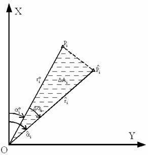
Figure 1: Reference datum in free network adjustment

Let now to insert the corrections from eq 10) in the first two relations of eq.(14):

and then dividing by k (number of points), we will obtain that the arithmetic mean of the coordinates after adjustment and before adjustment remains constant:

The last equation expresses nothing else that the geometrical center of the triangulation network remains fixed in free networks adjustment, in this way the absolute location of the network is implicitly established.

Now let start from eq. (19) where the adjusted coordinates are replaced using the same eq 10):

and making an extension in Taylor series around the approximate coordinates ()

The area swept by vector during the rotation between the two stages of free network adjustment with angle is:

Make a summation for all network points, the total area A becomes:

which reveals that the whole geodetic network has zero rotation during free network adjustment, although each individual radial vector from the origin to each point of the network may have undertaken a small rotation.

For the last relation given in eq 10), we consider the squared radial distances [see eq.(18)]:

Neglecting the second degree terms of the corrections:

Taking into account last row from eq 14)

which implies that the sum of all squared radial distances remains fixed in free network adjustment and the scale of the network is then defined.

4. Conclusions

From mathematical point of view, free network adjustment solution is perfectly demonstrated, using the minimum-norm least-squares inverse. Even in the networks with lacks sufficient reference datum the minimum-norm least-squares solution solves this problem somehow, but from geodetic point of view this is questionable because all four parameters (the origin of coordinate system, the orientation and the scale) are created artificially.

Free networks as trilateration networks or triangulation networks with some distance measurements do not lack scale datum, so the problem is reduced to establish the position and the orientation based on the first two upper conclusions.

The three dimensional free network can be viewed as the general case which includes even the 1D leveling networks as well as the 2D triangulation or/and trilateration networks. Photogrammetric bundle adjustment with relative orientation and without absolute orientation is one example where completely free 3D networks are involved [Papo, 1982].

5. References

[1] Andrei C.O., Analysis of geodetic networks using simulated observations. 2005, Department of Geodesy, Royal Institute of Technology, Stockholm, Sweden.

[2] Bjerhammar A., Theory of errors and Generalized Matrix Inverses. 1973, Elsevier, Amsterdam.

[3] Fan H., Theory of errors and Least Squares Adjustment. 2003, TRITA GEOD No. 2015, Department of Geodesy, Royal Institute of Technology, Stockholm, Sweden.

[4] Sjberg, L.E., Lecture Notes on General Matrix Calculus, Adjustment and Variance-Covariance Component Estimation. 1984, Nordiska forskarkurser "Optimization of Geodetic Operations". Norges Geogr.Oppm. Publ. 3/1984.

[5] Papo H.B., Perelmuter A., Free Net Analysis in Close-Range Photogrammetry. 1982, Photogrammetric Engineering and Remote Sensing, vol.48, No.4, pp.571-576.