| CATEGORII DOCUMENTE |
| Bulgara | Ceha slovaca | Croata | Engleza | Estona | Finlandeza | Franceza |
| Germana | Italiana | Letona | Lituaniana | Maghiara | Olandeza | Poloneza |
| Sarba | Slovena | Spaniola | Suedeza | Turca | Ucraineana |
Aggregate Demand and Aggregate Supply
![]()
WHATS NEW IN THE THIRD EDITION:
There is a new In the News box on 'The Trash Indicator' and a new Case Study on 'The 2001 Recession.' The Case Study on 'Oil and the Economy' has been updated. A new FYI box on 'The Origins of Aggregate Demand and Aggregate Supply' has also been added.
LEARNING OBJECTIVES:
By the end of this chapter, students should understand:
Ø three key facts about short-run economic fluctuations.
Ø how the economy in the short run differs from the economy in the long run.
Ø how to use the model of aggregate demand and aggregate supply to explain economic fluctuations.
Ø how shifts in either aggregate demand or aggregate supply can cause booms and recessions.
CONTEXT AND PURPOSE:
To this point, our study of macroeconomic theory has concentrated on the behavior of the economy in the long run. Chapters 20 through 22 now focus on short-run fluctuations in the economy around its long-term trend. Chapter 20 introduces aggregate demand and aggregate supply and shows how shifts in these curves can cause recessions. Chapter 21 focuses on how policymakers use the tools of monetary and fiscal policy to influence aggregate demand. Chapter 22 addresses the relationship between inflation and unemployment.
The purpose of Chapter 20 is to develop the model economists use to analyze the economys short-run fluctuationsthe model of aggregate demand and aggregate supply. Students will learn about some of the sources for shifts in the aggregate-demand curve and the aggregate-supply curve and how these shifts can cause recessions. This chapter also introduces actions policymakers might undertake to offset recessions.
KEY POINTS:
All societies experience short-run economic fluctuations around long-run trends. These fluctuations are irregular and largely unpredictable. When recessions do occur, real GDP and other measures of income, spending, and production fall, and unemployment rises.
Economists analyze short-run economic fluctuations using the model of aggregate demand and aggregate supply. According to this model, the output of goods and services and the overall level of prices adjust to balance aggregate demand and aggregate supply.
The aggregate-demand curve slopes downward for three reasons. First, a lower price level raises the real value of households money holdings, which stimulates consumer spending. Second, a lower price level reduces the quantity of money households demand; as households try to convert money into interest-bearing assets, interest rates fall, which stimulates investment spending. Third, as a lower price level reduces interest rates, the dollar depreciates in the market for foreign-currency exchange, which stimulates net exports.
Any event or policy that raises consumption, investment, government purchases, or net exports at a given price level increases aggregate demand. Any event or policy that reduces consumption, investment, government purchases, or net exports at a given price level decreases aggregate demand.
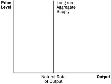
The long-run aggregate-supply curve is vertical. In the long run, the quantity of goods and services supplied depends on the economys labor, capital, natural resources, and technology, but not on the overall level of prices.
Three theories have been proposed to explain the upward slope of the short-run aggregate-supply curve. According to the sticky-wage theory, an unexpected fall in the price level temporarily raises real wages, which induces firms to reduce employment and production. According to the sticky-price theory, an unexpected fall in the price level leaves some firms with prices that are temporarily too high, which reduces their sales and causes them to cut back production. According to the misperceptions theory, an unexpected fall in the price level leads suppliers to mistakenly believe that their relative prices have fallen, which induces them to reduce production. All three theories imply that output deviates from its natural rate when the price level deviates from the price level that people expected.
Events that alter the economys ability to produce output, such as changes in labor, capital, natural resources, or technology shift the short-run aggregate supply curve (and may shift the long-run aggregate supply curve as well). In addition, the position of the short-run aggregate supply curve depends on the expected price level.
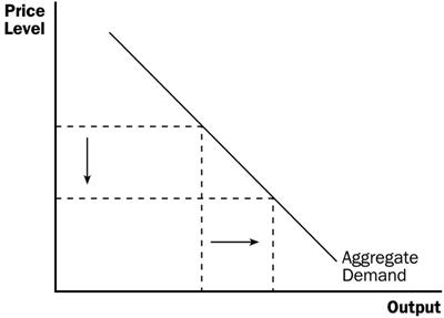
One possible cause of economic fluctuations is a shift in aggregate demand. When the aggregate-demand curve shifts to the left, output and prices fall in the short run. Over time, as a change in the expected price level causes perceptions, wages, and prices to adjust, the short-run aggregate-supply curve shifts to the right, and the economy returns to its natural rate of output at a new, lower price level.
A second possible cause of economic fluctuations is a shift in aggregate supply. When the aggregate-supply curve shifts to the left, the short-run effect is falling output and rising prices―a combination called stagflation. Over time, as perceptions, wages, and prices adjust, the price level falls back to its original level, and output recovers.
I. Economic activity fluctuates from year to year.
A. Definition of Recession: a period of declining real incomes and rising unemployment.
B. Definition of Depression: a severe recession.
II. Three Key Facts about Economic Fluctuations
Figure 1
A. Fact 1: Economic Fluctuations Are Irregular and Unpredictable
Fluctuations in the economy are often called the business cycle.
Economic fluctuations correspond to changes in business conditions.
These fluctuations are not at all regular and are almost impossible to predict.
Panel (a) of Figure 1 shows real GDP since 1965. The shaded areas represent recessions.
B. Fact 2: Most Macroeconomic Quantities Fluctuate Together
Real GDP is the variable that is most often used to examine short-run changes in the economy.
However, most macroeconomic variables that measure some type of income, spending, or production fluctuate closely together.
Panel (b) of Figure 1 shows how investment changes over the business cycle. Note that investment falls during recessions just as real GDP does.
C. Fact 3: As Output Falls, Unemployment Rises
Changes in the economys output level will have an effect on the economys utilization of its labor force.
When firms choose to produce a smaller amount of goods and services, they lay off workers, which increases the unemployment rate.
Panel (c) of Figure 1 shows how the unemployment rate changes over the business cycle. Note that during recessions, unemployment generally rises. Note also that the unemployment rate never approaches zero but instead fluctuates around its natural rate of about 5 percent.
D. In the News: The Trash Indicator
1. When the economy goes into a recession, many economic variables fall together.
2. This is an article from The Chicago Tribune discussing how the volume of trash generated by consumers is related to the health of the economy.
III. Explaining Short-Run Economic Fluctuations
A. How the Short Run Differs from the Long Run
Most economists believe that the classical theory describes the world in the long run but not in the short run.
Beyond a period of several years, changes in the money supply affect prices and other nominal variables, but do not affect real GDP, unemployment, or other real variables.
However, when studying year-to-year fluctuations in the economy, the assumption of monetary neutrality is not appropriate. In the short run, most real and nominal variables are intertwined.
B. The Basic Model of Economic Fluctuations
![]()
Definition of Model of Aggregate Demand and Aggregate Supply: the model that most economists use to explain short-run fluctuations in economic activity around its long-run trend.
We can show this model using a graph.
Figure 2
a. The variable on the vertical axis is the overall price level in the economy.
b. The variable on the horizontal axis is the overall quantity of goods and services.
c. Definition of Aggregate-Demand Curve: a curve that shows the quantity of goods and services that households, firms, and the government want to buy at each price level.
d. Definition of Aggregate-Supply Curve: a curve that shows the quantity of goods and services that firms choose to produce and sell at each price level.
In this model, the price level and the quantity of output adjust to bring aggregate demand and aggregate supply into balance.
IV. The Aggregate-Demand Curve
A. Why the Aggregate-Demand Curve Is Slopes Downward
Figure 3
Recall that GDP (Y) is made up of four components: consumption (C), investment (I), government purchases (G), and net exports (NX).
![]()
Each of the four components is a part of aggregate demand.
a. Government purchases are assumed to be fixed by policy.
b. This means that to understand why the aggregate-demand curve slopes downward, we must understand how changes in the price level affect consumption, investment, and net exports.

![]()

![]()
Table 1
The Price Level and Consumption: The Wealth Effect
a. A decrease in the price level makes consumers feel wealthier, which in turn encourages them to spend more.
b. The increase in consumer spending means a larger quantity of goods and services demanded.
The Price Level and Investment: The Interest-Rate Effect
a. The lower the price level, the less money households need to buy goods and services.
b. When the price level falls, households try to reduce their holdings of money by lending some out (either in financial markets or through financial intermediaries).
c. As households try to convert some of their money into interest-bearing assets, the interest rate will drop.
d. Lower interest rates encourage borrowing by firms that want to invest in new plants and equipment and by households who want to invest in new housing.
e. Thus, a lower price level reduces the interest rate, encourages greater spending on investment goods, and therefore increases the quantity of goods and services demanded.
5. The Price Level and Net Exports: The Exchange-Rate Effect
a. A lower price level in the
b. American investors will seek higher
returns by investing abroad, increasing
c. The increase in net capital outflow raises the supply of dollars, lowering the real exchange rate.
d.
e. Therefore, when a fall in the
6. All three of these effects imply that, all else equal, there is an inverse relationship between the price level and the quantity of goods and services demanded.

![]()
B. Why the Aggregate-Demand Curve Might Shift
![]()
Shifts Arising from Consumption
a. If Americans become more concerned with saving for retirement and reduce current consumption, aggregate demand will decline.
b. If the government cuts taxes, it encourages people to spend more, resulting in an increase in aggregate demand.
2. Shifts Arising from Investment
a. Suppose that the computer industry introduces a faster line of computers and many firms decide to invest in new computer systems. This will lead to an increase in aggregate demand.
b. If firms become pessimistic about future business conditions, they may cut back on investment spending, shifting aggregate demand to the left.
c. An investment tax credit increases the quantity of investment goods that firms demand, which results in an increase in aggregate demand.
d. An increase in the supply of money lowers the interest rate in the short run. This lead to more investment spending, which causes an increase in aggregate demand.
3. Shifts Arising from Government Purchases
a. If Congress decides to reduce purchases of new weapon systems, aggregate demand will fall.
b. If state governments decide to build more state highways, aggregate demand will shift to the right.
4. Shifts Arising from Net Exports
a. When
b. If the exchange rate of the U.S. dollar
increases,
V. The Aggregate-Supply Curve
Figure 4
A. The relationship between the price level and the quantity of goods and services supplied depends on the time horizon being examined.
B. Why the Aggregate-Supply Curve Is Vertical in the Long Run
In the long run, an economys production of goods and services depends on its supplies of resources along with the available production technology.
Because the price level does not affect these determinants of output in the long run, the long-run aggregate-supply curve is vertical.
C. Why the Long-Run Aggregate-Supply Curve Might Shift
The position of the aggregate supply curve occurs at an output level sometimes referred to as potential output or full-employment output.
This is the level of output that the economy produces when unemployment is at its natural rate.
Any change in the economy that alters the natural rate of output shifts the long-run aggregate-supply curve.
Shifts Arising from Labor
a. Increases in immigration increase the number of workers available. The long-run aggregate-supply curve would shift to the right.
b. Any change in the natural rate of unemployment will alter long-run aggregate supply as well.
5. Shifts Arising from Capital
a. An increase in the economys capital stock raises productivity and thus shifts long-run aggregate supply to the right.
b. This would also be true if the increase occurred in human capital rather than physical capital.
6. Shifts Arising from Natural Resources
a. A discovery of a new mineral deposit increases long-run aggregate supply.
b. A change in weather patterns that makes farming more difficult shifts long-run aggregate supply to the left.
c. A change in the availability of imported resources can also affect long-run aggregate supply.
7. Shifts Arising from Technological Knowledge
a. The invention of the computer has allowed us to produce more goods and services from any given level of resources. As a result, it has shifted the long-run aggregate-supply curve to the right.
b. Opening up international trade has similar effects to inventing new production processes. Therefore, it also shifts the long-run aggregate-supply curve to the right.
D. A New Way to Depict Long-Run Growth and Inflation
Figure 5
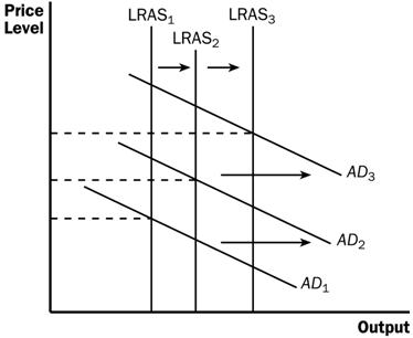
Two important forces that govern the economy in the long run are technological progress and monetary policy.
a. Technological progress shifts long-run aggregate supply to the right.
b. The Fed increases the money supply over time, which raises aggregate demand.
The result is growth in output and continuing inflation (increases in the price level).
Although the purpose of developing the aggregate demand/aggregate supply model is to describe short-run fluctuations, these short-run fluctuations should be considered to be deviations from the continuing long-run trends developed here.
E. Why the Aggregate-Supply Curve Is Upward Sloping in the Short Run
Table 2
Figure 6
The Sticky-Wage Theory
a. Nominal wages are often slow to adjust in the economy due to long-term contracts between workers and firms.
b. Example: Suppose a firm has agreed in advance to pay workers a certain amount and then the price level falls unexpectedly. This implies that the firm is now paying a real wage that is larger than it intended, raising the costs of production. Thus, the firm hires less labor and produces a smaller quantity of goods and services.
c. Therefore, because wages do not immediately adjust to the price level, a lower price level makes employment and production less profitable, leading firms to lower the quantity of goods and services supplied.
The Sticky-Price Theory
a. The prices of some goods and services are also sometimes slow to respond to changes in the economy. This is often blamed on menu costs.
b. If the price level falls unexpectedly, and a firm does not change the price of its product quickly, its relative price will rise and this will lead to a loss in sales.
c. Thus, when sales decline, firms will produce a lower quantity of goods and services.
d. Because not all prices adjust instantly to changing conditions, an unexpected fall in the price level leaves some firms with higher-than-desired prices, which depress sales and cause firms to lower the quantity of goods and services supplied.
The Misperceptions Theory
a. Changes in the overall price level can temporarily mislead suppliers about what is happening in the markets in which they sell their output.
b. As a result of these misperceptions, suppliers respond to changes in the level of prices and thus, the short-run aggregate-supply curve is upward sloping.
c. Example: The price level falls unexpectedly. Suppliers mistakenly believe that as the price of their product falls, it is a drop in the relative price of their product. Suppliers may then believe that the reward of supplying their product has fallen, and thus they decrease the quantity that they supply. The same misperception may happen if workers see a decline in their nominal wage (caused by a fall in the price level).
d. Thus, a lower price level causes misperceptions about relative prices, and these misperceptions lead suppliers to respond to the lower price level by decreasing the quantity of goods and services supplied.
Note that each of these theories suggest that output deviates from its natural rate when the price level deviates from the price level that people expected.
5. Note also that the effects of the change in the price level will be temporary. Eventually people will adjust their price level expectations and output will return to its natural level; thus, the aggregate-supply curve will be vertical in the long run.
F. Why the Short-Run Aggregate-Supply Curve Might Shift
Events that shift the long-run aggregate-supply curve will shift the short-run aggregate-supply curve as well.
However, peoples expectations of the price level will affect the position of the short-run aggregate-supply curve even though it has no effect on the long-run aggregate-supply curve.
A higher expected price level decreases the quantity of goods and services supplied and shifts the short-run aggregate-supply curve to the left. A lower expected price level increases the quantity of goods and services supplied and shifts the short-run aggregate-supply curve to the right.
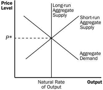
VI. Two Causes of Economic Fluctuations
A. Long-Run Equilibrium
Figure 7
Long-run equilibrium is found where the aggregate-demand curve intersects with the long-run aggregate-supply curve.
Output is at its natural rate.
Also at this point, perceptions, wages, and prices have all adjusted so that the short-run aggregate-supply curve intersects at this point as well.
B. The Effects of a Shift in Aggregate Demand
Figure 8

![]()
Example: Pessimism causes household spending and investment to decline.
This will cause the aggregate demand curve to shift to the left.
In the short run, both output and the price level fall. This drop in output means that the economy is in a recession.
It is possible that policymakers may want to eliminate the recession by boosting government spending or increasing the money supply. Either way, these policies could shift the aggregate demand curve back to the right.
5. However, even if policymakers do nothing, the economy will eventually move back to the natural rate of output.
a. People will correct the misperceptions, sticky wages, and sticky prices that cause the aggregate-supply curve to be upward sloping in the short run.
b. The expected price level will fall, shifting the short-run aggregate-supply curve to the right.
6. In the long run, the decrease in aggregate demand can be seen solely by the drop in the equilibrium price level. Thus, the long-run effect of a change in aggregate demand is a nominal change (in the price level) but not a real change (output is the same).
7. Case Study: Two Big Shifts in Aggregate Demand: The Great Depression and World War II
Figure 9
a. Figure
9 shows real GDP for the
b. Two time periods of economic fluctuations can be seen dramatically in the picture. These are the early 1930s (the Great Depression) and the early 1940s (World War II).
c. From 1929 to 1933, GDP fell by 27 percent. From 1939 to 1944, the economys production of goods and services almost doubled.
8. Case Study: The Recession of 2001
a. The
b. The recession has been attributed to three aggregate demand shocks. First, the dot.com bubble in the stock market ended. Second, the terrorist attack in September 2001 led to increased uncertainty. Third, several corporate accounting scandals were revealed.
c. The federal government passed tax cuts to improve consumer spending, while the Fed responded by keeping interest rates low.
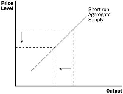
C. The Effects of a Shift in Aggregate Supply
Figure 10
Example: Firms experience a sudden increase in their costs of production.
This will cause the short-run aggregate-supply curve to shift to the left. (Depending on the event, long-run aggregate supply may also shift. We will assume that it does not.)
![]()
In the short run, output will fall and the price level will rise. The economy is experiencing stagflation.
Definition of stagflation: a period of falling output and rising prices.
Figure 11
5. Policymakers will have a more difficult time with this situation. Policymakers can shift the aggregate-demand curve, but cannot simultaneously offset the drop in output and the rise in the price level. If they increase aggregate demand, the recession will end, but the price level will be permanently higher.
6. If policymakers do nothing, price expectations will adjust, causing the short-run aggregate-supply curve to shift back to the right.
7. Case Study: Oil and the Economy
a. Crude oil is a key input in the production of many goods and services.
b. When some event (often political) leads to a rise in the price of crude oil, firms must endure higher costs of production and the short-run aggregate-supply curve shifts to the left.
c. In the mid-1970s, OPEC lowered
production of oil and the price of crude oil rose substantially. The inflation rate in the
d. This occurred again in the late 1970s. Oil prices rose, output fell, and the rate of inflation increased.
e. In the late 1980s, OPEC began to lose control over the oil market as members began cheating on the agreement. Oil prices fell, which led to a rightward shift of the short-run aggregate supply curve. This caused both unemployment and inflation to decline.
f. In recent years, the world market for oil has not been as important a source of economic fluctuations.
VII. FYI: The Origins of Aggregate Demand and Aggregate Supply
A. The AD/AS model is a by-product of the Great Depression.
B. In 1936, economist John Maynard Keynes published a book that attempted to explain short-run fluctuations.
C. Keynes believed that recessions occur because of inadequate demand for goods and services.
D. Therefore, Keynes advocated policies to increase aggregate demand.
Activity 1 National Income Article Type: Take-home
assignment Topics: Fluctuations in
output and the price level Class
limitations: Works in
any class Purpose This
assignment is a good way for students to connect economic theory to actual
events. Assignment Find an article in a recent newspaper
or magazine illustrating a change that will affect National Income. Analyze the situation using economic
reasoning. Draw an Aggregate Demand and Aggregate
Supply graph to explain this change. Be sure to label your graph and
clearly indicate which curve shifts. Explain what happens to National
Income and to the price level in the short run. Turn in a copy of the article along
with your explanation. Points for Discussion This can
be a nice way to review the elements of Aggregate Demandconsumption,
investment, government spending, and net exportsand the elements of
Aggregate Supplyproductive resources, technology. Most
changes will only shift one curve. Discussing
the long-run impact of these changes can emphasize the differences between
AS and AD shifts.
Activity 2 The Economics of War Type: In-class
assignment Topics: National Income,
price levels, total spending, resources Materials
needed: None Time: 20 minutes Class
limitations: Works in
any size class Purpose This
assignment asks students to examine their beliefs about the impact of war
on the economy. It can be used to
examine aggregate demand shifts and aggregate supply shifts. This
assignment can generate lively discussion. Instructions Ask the class to answer the following questions. Give
them time to write an answer to a question, then discuss their answers
before moving to the next question. Is war good or bad for the economy? What are the opportunity costs of using
resources in wars? How would a war affect aggregate
supply?
Graph the shift in aggregate supply.
What happens to output and the price level? How would a war affect aggregate
demand? Graph the shift in aggregate demand.
What happens to output and the price level? Is peace good or bad for the economy? Common Answers and Points for Discussion Is war good
or bad for the economy? A surprising number of students say
war is goodmany use WWII and its stimulative impact on the What are the opportunity costs of using
resources in wars? Lost civilian production is an important
opportunity cost. Rationing, price controls, and black markets are common
in time of war. In poor countries, shifting resources from consumption to
military use can lead to starvation. People displaced by fighting will be
unlikely to continue their regular activitiescausing unemployment. Any
resources destroyed in the wardeaths, bombed factories or bridges, burned
cropswill be unavailable for any use. How would a war affect aggregate
supply? This question has a variety of
correct answers. The resources destroyed by war are unavailable for
productive purposes. This would decrease aggregate supply. Some wars begin
as attempts to seize resourcesmore land, mines, petroleum reserves. If
this is successful, it increases the aggregate supply of the winning
country, but reduces that of the losing country. If countries develop new
technologies, or invest in strategic industries, aggregate supply could
increase. Graph the shift in aggregate supply.
What happens to output and the price level? If aggregate supply decreases,
output falls and the price level rises. If aggregate supply increases,
output rises and the price level falls. How would a war affect aggregate
demand? This question also has several
answers. In many cases, high levels of military spending will increase
aggregate demand. In areas where fighting is active, other spending sectors
will be suppressedless consumption, less investment, and perhaps a
decrease in international trade. This would decrease aggregate demand. Graph the shift in aggregate demand.
What happens to output and the price level? An increase in aggregate demand will
stimulate the economy in the short runoutput increases, as does the price
level. Wars often are associated with inflation, but low levels of
unemployment. Is peace good or bad for the economy? In general, periods of prosperity
are also periods of peace. Markets are allowed to put resources to their
highest and best uses. Of course, as Keynes pointed out, military
expenditures can be an important component of total spending. Sudden
decreases in government spending can lead to recession and unemployment.
SOLUTIONS TO TEXT PROBLEMS:
Quick Quizzes
1. Three key facts about economic fluctuations are: (1) economic fluctuations are irregular and unpredictable; (2) most macroeconomic quantities fluctuate together; and (3) as output falls, unemployment rises.
Economic fluctuations are irregular and unpredictable, as you can see by looking at a graph of real GDP over time. Some recessions are close together and others are far apart. There appears to be no recurring pattern.
Most macroeconomic quantities fluctuate together. In recessions, real GDP, consumer spending, investment spending, corporate profits, and other macroeconomic variables decline or grow much more slowly than during economic expansions. However, the variables fluctuate by different amounts over the business cycle, with investment varying much more than other variables.
As output falls, unemployment rises, because when firms want to produce less, they do so by laying off workers, thus causing a rise in unemployment.
2. The economys behavior in the short run differs from its behavior in the long run because the assumption of monetary neutrality applies to the long run, not the short run. In the short run, real and nominal variables are highly intertwined.
Figure 1 shows the model of aggregate demand and aggregate supply. The horizontal axis shows the quantity of output and the vertical axis shows the price level.
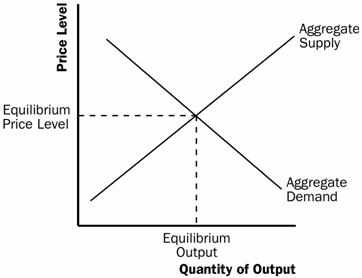
Figure 1
3. The aggregate-demand curve slopes downward for three reasons. First, when prices fall, the value of dollars in peoples wallets and bank accounts rises, so they are wealthier. As a result, they spend more, so aggregate demand increases. Second, when prices fall, people need less money to make their purchases, so they lend more out, which reduces the interest rate. The lower interest rate encourages businesses to invest more, raising aggregate demand. Third, since lower prices lead to a lower interest rate, investors move money from domestic investment to foreign investment, supplying dollars to the foreign-exchange market, thus causing the dollar to depreciate. The decline in the real exchange rate causes net exports to increase, which raises aggregate demand.
Any event that alters the level of consumption, investment, government purchases, or net exports at any price level will lead to a shift in aggregate demand. An increase in expenditure will shift the aggregate demand curve to the right, while a decline in expenditure will shift the aggregate demand curve to the left.
4. The long-run aggregate-supply curve is vertical because the price level does not affect the long-run determinants of real GDP, which include supplies of labor, capital, natural resources, and the level of available technology. This is just an application of the classical dichotomy and monetary neutrality.
There are three reasons why the short-run aggregate-supply curve slopes upward. First, the sticky-wage theory suggests that because nominal wages are slow to adjust, a decline in the price level means real wages are higher, so firms hire fewer workers and produce less, causing aggregate supply to decline. Second, the sticky-price theory suggests that the prices of some goods and services are slow to change. Then, if some economic event causes the overall price level to decline, prices that are sticky wont be able to adjust immediately, so relative prices of those goods will rise and the demand for those goods will decline, leading firms to cut back on production. Thus, lower overall prices lead to lower aggregate supply. Third, the misperceptions theory suggests that changes in the overall price level can temporarily mislead suppliers. When the price level falls below the level that was expected, suppliers think that the relative prices of their products have declined, so they produce less. Thus, a lower price level reduces aggregate supply.
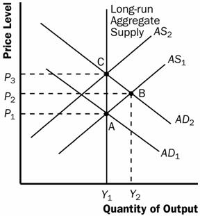
Figure 2
When a popular presidential candidate is elected, causing people to be more confident about the future, they will spend more, causing the aggregate-demand curve to shift to the right, as shown in Figure 2. The economy begins at point A with aggregate-demand curve AD1 and short-run aggregate-supply curve AS1. The equilibrium has price level P1 and output level Y1. Increased confidence about the future causes the aggregate-demand curve to shift to AD2. Now the economy is at point B, with price level P2 and output level Y2. Over time, the short-run aggregate-supply curve shifts up to AS2 and the economy gets to equilibrium at point C, with price level P3 and output level Y1.
Questions for Review
1. Two macroeconomic variables that decline when the economy goes into a recession are real GDP and investment spending (many other answers are possible). A macroeconomic variable that rises during a recession is the unemployment rate.
Figure 3 shows aggregate demand, short-run aggregate supply, and long-run aggregate supply.
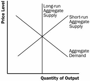
Figure 3
The aggregate-demand curve is downward sloping because: (1) a decrease in the price level makes consumers feel wealthier, which in turn encourages them to spend more, so there is a larger quantity of goods and services demanded; (2) a lower price level reduces the interest rate, encouraging greater spending on investment, so there is a larger quantity of goods and services demanded; (3) a fall in the U.S. price level causes U.S. interest rates to fall, so the real exchange rate depreciates, stimulating U.S. net exports, so there is a larger quantity of goods and services demanded.
The long-run aggregate supply curve is vertical because in the long run, an economy's supply of goods and services depends on its supplies of capital, labor, and natural resources and on the available production technology used to turn these resources into goods and services. The price level does not affect these long-run determinants of real GDP.
Three theories explain why the short-run aggregate-supply curve is upward sloping:
(1) the sticky-wage theory, in which a lower price level makes employment and production less profitable because wages do not adjust immediately to the price level, so firms reduce the quantity of goods and services supplied; (2) the sticky-price theory, in which an unexpected fall in the price level leaves some firms with higher-than-desired prices because not all prices adjust instantly to changing conditions, which depresses sales and induces firms to reduce the quantity of goods and services they produce; and (3) the misperceptions theory, in which a lower price level causes misperceptions about relative prices, and these misperceptions induce suppliers to respond to the lower price level by decreasing the quantity of goods and services supplied.
6. The aggregate-demand curve might shift to the left when something (other than a rise in the price level) causes a reduction in consumption spending (such as a desire for increased saving), a reduction in investment spending (such as increased taxes on the returns to investment), decreased government spending (such as a cutback in defense spending), or reduced net exports (such as when foreign economies go into recession, so our exports fall.
Figure 4 traces through the steps of such a shift in aggregate demand. The economy begins in equilibrium, with short-run aggregate supply, AS1, intersecting aggregate demand, AD1, at point A. When the aggregate-demand curve shifts to the left to AD2, the economy moves from point A to point B, reducing the price level and the quantity of output. Over time, people adjust their perceptions, wages, and prices, shifting the short-run aggregate-supply curve down to AS2, and moving the economy from point B to point C, which is back on the long-run aggregate supply curve and has a lower price level.
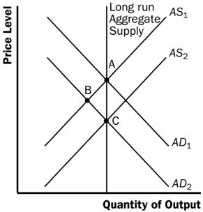
Figure 4
The aggregate-supply curve might shift to the left because of a decline in the economy's capital stock, labor supply, or productivity, or an increase in the natural rate of unemployment, all of which shift both the long-run and short-run aggregate supply curves to the left. An increase in the expected price level shifts just the short-run aggregate-supply curve (not the long-run aggregate-supply curve) to the left.
Figure 5 traces through the effects of such a shift. The economy starts in equilibrium at point A. The aggregate-supply curve then shifts to the left from AS1 to AS2. The new equilibrium is at point B, the intersection of the aggregate-demand curve and AS2. As time goes on, the economy returns to long-run equilibrium at point A, as the short-run aggregate supply curve shifts back to its original position.
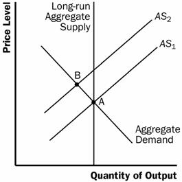
Figure 5
Problems and Applications
Investment is more variable than consumer spending over the business cycle because firms can curtail investment spending more easily than households can curtail consumption spending. In recessions, firms know they will not be able to sell as many goods, so they want to produce less and therefore they put off buying capital (they do not expand factories or buy new equipment). Much of consumer spending is on necessities, like food, which cannot decline as much in recessions. So, investment spending is more variable over the business cycle than consumer spending. For similar reasons, durable goods spending is the most volatile sector of consumer spending. Durable goods, such as furniture and car purchases, are more volatile over the business cycle than nondurable goods, such as food and clothing, or services, such as haircuts and medical care, for the same reason. People put off buying durable goods and just make do with older cars and furniture when economic times are bad.
2. a. The current state of the economy is shown in Figure 6. The aggregate-demand curve and short-run aggregate-supply curve intersect at a point to the left of long-run aggregate supply.
b. A stock market crash leads to a leftward shift of aggregate demand. The equilibrium level of output and the price level will fall. Since the quantity of output is less than the natural rate of output, the unemployment rate will rise above the natural rate of unemployment.
c. If nominal wages are unchanged as the price level falls, firms will be forced to cut back on employment and production. Over time as expectations adjust, the short-run aggregate supply curve will shift to the right moving the economy back to the natural rate of output.
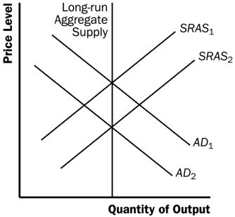
Figure 6
3. a. When the United States experiences a wave of immigration, the labor force increases, so long-run aggregate supply increases as there are more people who can produce output.
b. When Congress raises the minimum wage to $10 per hour, the natural rate of unemployment rises, so the long-run aggregate-supply curve shifts to the left.
c. When Intel invents a new and more powerful computer chip, productivity increases, so long-run aggregate supply increases as more output can be produced with the same inputs.
d. When a severe hurricane damages factories along the East Coast, the capital stock is smaller, so long-run aggregate supply declines.
In Figure 8 in the textbook, the unemployment rate at point B is higher than the unemployment rate at point A because output is lower at B than at A. The unemployment rate at point C is the same as that at point A because output is the same at both points. According to the sticky-wage explanation of the short-run aggregate supply curve, output is lower at point B than at point A because wages have not adjusted. The nominal wage at points A and B are the same, but since the price level is lower at point B the real wage is higher, so firms hire fewer workers and thus output is lower. Point C is on the long-run aggregate supply curve, as is point A, so the real wage must be the same at the two points. Since the price level is lower at point C, the nominal wage at point C must be lower.
5. a. The statement that 'the aggregate-demand curve slopes downward because it is the horizontal sum of the demand curves for individual goods' is false. The aggregate-demand curve slopes downward because a fall in the price level raises the overall quantity of goods and services demanded through the wealth effect, the interest-rate effect, and the exchange-rate effect.
b. The statement that 'the long-run aggregate-supply curve is vertical because economic forces do not affect long-run aggregate supply' is false. Economic forces of various kinds (such as population and productivity) do affect long-run aggregate supply. The long-run aggregate-supply curve is vertical because the price level does not affect long-run aggregate supply.
c. The statement that 'if firms adjusted their prices every day, then the short-run aggregate-supply curve would be horizontal' is false. If firms adjusted prices quickly and if sticky prices were the only possible cause for the upward slope of the short-run aggregate supply curve, then the short-run aggregate-supply curve would be vertical, not horizontal. The short-run aggregate supply curve would be horizontal only if prices were completely fixed.
d. The statement that 'whenever the economy enters a recession, its long-run aggregate-supply curve shifts to the left' is false. An economy could enter a recession if the aggregate-demand curve or the short-run aggregate-supply curve shift to the left.
6. a. According to the sticky-wage theory, the economy is in a recession because the price level has declined so that real wages are too high, thus labor demand is too low. Over time, as nominal wages are adjusted so that real wages decline, the economy returns to full employment.
According to the sticky-price theory, the economy is in a recession because not all prices adjust quickly. Over time, firms are able to adjust their prices more fully, and the economy returns to the long-run aggregate-supply curve.
According to the misperceptions theory, the economy is in a recession when the price level is below what was expected. Over time, as people observe the lower price level, their expectations adjust, and the economy returns to the long-run aggregate-supply curve.
b. The speed of the recovery in each theory depends on how quickly price expectations, wages, and prices adjust.
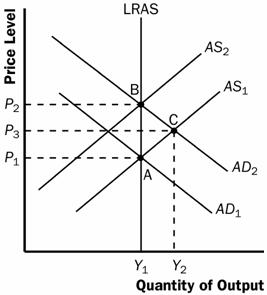
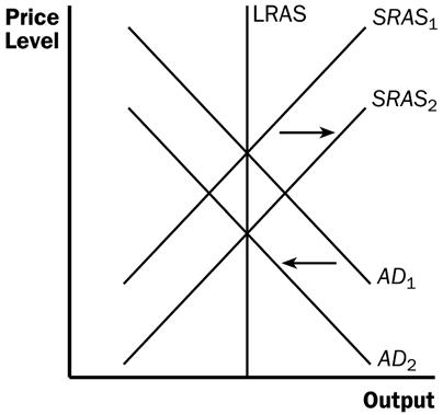
Figure 7
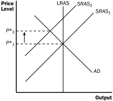
7. If the Fed increases the money supply and people expect a higher price level, the aggregate-demand curve shifts to the right and the short-run aggregate-supply curve shifts to the left, as shown in Figure 7. The economy moves from point A to point B, with no change in output and a rise in the price level (to P2). If the public does not change its expectation of the price level, the short-run aggregate-supply curve does not shift, the economy ends up at point C, and output increases along with the price level (to P3).
Figure 8 depicts an economy in a recession. The short-run aggregate supply curve is AS1 and the economy is at equilibrium at point A, which is to the left of the long-run aggregate-supply curve. If policymakers take no action, the economy will return to the long-run aggregate-supply curve over time as the short-run aggregate-supply curve shifts to the right to AS2. The economy's new equilibrium is at point B.
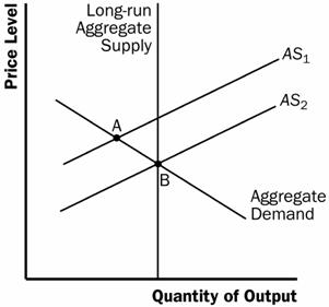
Figure 8
a. If people believe that inflation will be high over the next year, workers will want higher nominal wages. If the price level does not rise as much as wages do, real wages will increase, so firms will not hire as many workers.
b. Figure 9 shows the economy starting out at point A on short-run aggregate-supply curve AS1. With higher nominal wages, the short-run aggregate-supply curve will shift to the left to AS2. The new equilibrium is at point B, with output less than long-run aggregate supply. In the short run, the price level rises and output falls. In the long-run, the economy will return to point A, as the decline in output eventually leads to a decline in the price level and the short-run aggregate-supply curve returns to AS1.
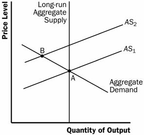
Figure 9
c. In the short-run, expectations of higher inflation were somewhat accurate, as the price level is higher at point B than at point A (however, the price level at point B is not as high as was expected). But inflation expectations were wrong in the long run.
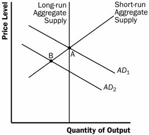
Figure 10
a. If households decide to save a larger share of their income, they must spend less on consumer goods, so the aggregate-demand curve shifts to the left, as shown in Figure 10. The equilibrium changes from point A to point B, so the price level declines and output declines.
b. If
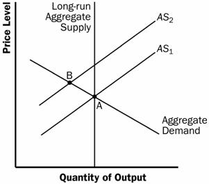
Figure 11
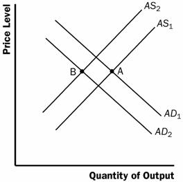
Figure 12
c. If increased job opportunities cause people to leave the country, the short-run aggregate-supply curve will shift to the left because there are fewer people producing output. The aggregate-demand curve will shift to the left because there are fewer people consuming goods and services. The result is a decline in the quantity of output, as Figure 12 shows. Whether the price level rises or declines depends on the size of the shifts in the aggregate-demand curve and the short-run aggregate-supply curve.
a. When the stock market declines sharply, wealth declines, so the aggregate-demand curve shifts to the left, as shown in Figure 13. In the short run, the economy moves from point A to point B, as output declines and the price level declines. In the long run, the short-run aggregate-supply curve shifts to the right to restore equilibrium at point C, with unchanged output and a lower price level compared to point A.
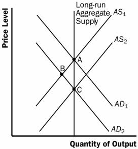
Figure 13

Figure 14
b. When the federal government increases spending on national defense, the rise in government purchases shifts the aggregate-demand curve to the right, as shown in Figure 14. In the short run, the economy moves from point A to point B, as output and the price level rise. In the long run, the short-run aggregate-supply curve shifts to the left to restore equilibrium at point C, with unchanged output and a higher price level compared to point A.
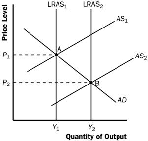
Figure 15
c. When a technological improvement raises productivity, the long-run and short-run aggregate-supply curves shift to the right, as shown in Figure 15. The economy moves from point A to point B, as output rises and the price level declines.

Figure 16
d. When a recession overseas causes
foreigners to buy fewer
a. If firms become optimistic about future business conditions and invest a lot, the result is shown in Figure 17. The economy begins at point A with aggregate-demand curve AD1 and short-run aggregate-supply curve AS1. The equilibrium has price level P1 and output level Y1. Increased optimism leads to greater investment, so the aggregate-demand curve shifts to AD2. Now the economy is at point B, with price level P2 and output level Y2. The aggregate quantity of output supplied rises because the price level has risen and people have misperceptions about the price level, wages are sticky, or prices are sticky, all of which cause output supplied to increase.
b. Over time, as the misperceptions of the price level disappear, wages adjust, or prices adjust, the short-run aggregate-supply curve shifts up to AS2 and the economy gets to equilibrium at point C, with price level P3 and output level Y1. The quantity of output demanded declines as the price level rises.
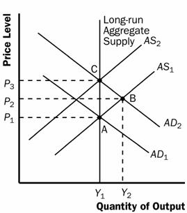
Figure 17
c. The investment boom might increase the long-run aggregate-supply curve because higher investment today means a larger capital stock in the future, thus higher productivity and output.
The idea of lengthening the shopping period between Thanksgiving and Christmas was to increase aggregate demand. As Figure 18 shows, this could increase output back to its long-run equilibrium level.
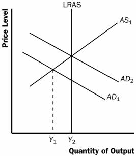
Figure 18
Many answers are possible.
|
Politica de confidentialitate | Termeni si conditii de utilizare |

Vizualizari: 3311
Importanta: ![]()
Termeni si conditii de utilizare | Contact
© SCRIGROUP 2024 . All rights reserved