| CATEGORII DOCUMENTE |
| Asp | Autocad | C | Dot net | Excel | Fox pro | Html | Java |
| Linux | Mathcad | Photoshop | Php | Sql | Visual studio | Windows | Xml |
DOCUMENTE SIMILARE |
||||
|
||||
Excel contains several SUM functions, which extend your capabilities far beyond the simple summing of a group of numbers in a range of cells. Even the lowly SUM function can take arguments. Listed below are the SUM functions found in the Excel package.
Thankfully, most of these functions are used by statisticians; we won't often find a need for them. A couple, however, are important enough to know for everyday use. In this section, we will look at SUM and SUMIF, and touch briefly on SUMPRODUCT.
|
Function |
Description |
|
SUM |
Adds all the numbers in a range of cells. |
|
SUMIF |
Adds the cells specified by a given criteria. |
|
SUMPRODUCT |
Multiplies corresponding components in given arrays, and returns the sum of those products. |
|
SUMSQ |
Returns the sum of the squares of the arguments. |
|
SUMX2MY2 |
Returns the sum of the difference of squares of corresponding values in two arrays. |
|
SUMX2PY2 |
Returns the sum of the sum of squares corresponding values in two arrays. (The sum of the sum of squares is a common term in many statistical calculations.) |
|
SUMXMY2 |
Returns the sum of squares of differences corresponding values in two arrays. |
SUM
The SUM function is straightforward, and you probably use it every day to add ranges of numbers to produce a total. It works as you would expect it to -- until you begin to add arguments to it. For example, take a look at this:
=SUM('3',3,TRUE)The above statement evaluates to 7 when entered in the worksheet. You can see an example of this on Sheet 5 in your workbook. Look at cell I2, under Points of Interest. In order for the formula shown above to evaluate to 7, what must happen? The text value of '3' is converted to a numeric value, and TRUE is evaluated as 1. Now, if you look at Sheet 5, you see '3' in H4, 3 in H5, and TRUE in H6. In I7, we developed the formula below:
Now in cell I7, you see the value 3. What happened this time? In other words, what did we do differently that caused Excel to behave differently? The answer is that in the second version, we used cell references in the formula instead of the literal values. The lesson to keep in mind is that when you use cell references with this type of formula, Excel does not convert the cell entries from their native type -- it will ignore invalid types.
This function takes arguments and tests a cell to see if the argument is met. If the argument returns TRUE, then the value found in the cell is included in the SUM result. Here's the syntax of the SUMIF function:
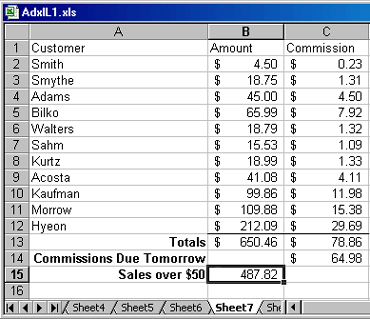
=SUMIF(range, criteria, sum_range)The sum_range is an optional argument to the function. If left out, SUMIF will sum the matching values in range. See Sheet 6 in the workbook for this lesson to see how SUMIF operates. In the example, a series of sales amounts are shown in cells B2:B12. Commissions on sales are shown in cells C2:C12. Assume it is the store's policy to pay sales commissions on items over $50 the next day. We need to know our total commissions payable. The answer is found with SUMIF. The formula, input in cell C14, looks like this:
=SUMIF(B2:B12,'>=50',C2:C12)Note the quotation marks around the criteria. They are required because of the >= symbols. The formula won't work without them. Go now to Sheet 7 in your workbook, and try building the SUMIF for sales greater than $50 in cell C14. In cell B15, use SUMIF without the sum range entry and see what happens. Your completed worksheet will look like the sample below:

Figure 1-7: The completed worksheet.
SUMPRODUCT
This function multiplies the corresponding components in the given arrays and returns the sum of those products. The syntax of this command is:
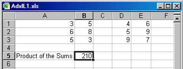
=SUMPRODUCT(array1, array2, array3, array4, )A minimum of two arrays is required for the function to work. Let's use this function on the array shown in the sample below:

Figure 1-8: Two arrays of the same dimension.
The result of SUMPRODUCT is derived through the following process: 3*4+5*6+6*5+8*9+5*9+3*7. The same result can be obtained by typing the matrix values into the SUMPRODUCT formula as follows:
=SUMPRODUCT(, )Although you can type the matrix values into the formula, it's easier to enter these values directly into the cells of the worksheet. In the following example, the same result is derived using the formula:
=SUMPRODUCT(A1:B3*D1:E3)Matrices are often used to solve complex business problems, and we will be looking at more scenarios using matrix functions later in this course.
Go to Sheet 8 now and construct the SUMPRODUCT formula in cell B5. The result you see needs to match the result in the figure above.
a note about SUMPRODUCT
Array1, array2, array3 . . . are 2 to 30 arrays whose components you need to multiply and then add. The arrays must have the same dimensions. When they do not, Excel returns the #VALUE! error. SUMPRODUCT treats entries that are not numeric as if they are zeros.
|
Politica de confidentialitate | Termeni si conditii de utilizare |

Vizualizari: 1449
Importanta: ![]()
Termeni si conditii de utilizare | Contact
© SCRIGROUP 2025 . All rights reserved