| CATEGORII DOCUMENTE |
| Bulgara | Ceha slovaca | Croata | Engleza | Estona | Finlandeza | Franceza |
| Germana | Italiana | Letona | Lituaniana | Maghiara | Olandeza | Poloneza |
| Sarba | Slovena | Spaniola | Suedeza | Turca | Ucraineana |
DicomTools, which this paper is about, is a customized, 3D visualization application created with the goal of visualizing in 3D the human brain aiding the surgeon to study the brain of the patient and prepare for brain surgery. More formally speaking it is a stereotactic planner and diagnosis tool.
It processes mainly DICOM (Digital Imaging and Communications in Medicine) image files, but it can read also other common image formats.
Among many things it can visualize medical volumes in three dimensions, realize orthogonal and oblique reslicing, segmentation, relative and absolute targeting; read, group, sort, anonymize DICOM files and create realistic models of human brain structures.
It is realized using several image processing algorithms and visualization techniques. It uses the free source libraries VTK (Visualization Toolkit), an ITK (Insight Registration and Segmentation Toolkit).
DicomTools is capable of visualizing and processing almost any kind of human or animal body part or organ, but it is tuned especially for the human brain and in particular for a deep brain simulation operation.
This research project was made in collaboration with the firm
Their main goal is to develop and manufacture hardware and software systems for functional neurosurgery and fundamental neuroscience, with an emphasis on invasive electrophysiological brain mapping, data analysis and multi-information rendering. [Neurostar]
The chief coordinator of the research team was Dr. Med. Sorin Breit from the Neurosurgery Clinic of Tuebingen, the lead coordinator of the software team being Radu C. Popa, the coordinator of the local team of Cluj-Napoca being Pter Horvth and I also worked together on the project with a student from the Technical University of Cluj-Napoca, Roxana Racz who did the image registration and fusion part of DicomTools.
Deep Brain Stimulation is a relatively old technique for treatment of moving disorders like Parkinsons disease, tremors, epilepsy and chronic pain.
Parkinson's disease is a neurological disorder that erodes a person's control over their movements and speech. Over one million Americans suffers from this slowly progressive, debilitating disease. [UMM01]
Alternate solutions for treating this type of movement disorders are ablation and medicines.
Unfortunately these techniques have proven to have undesirable side effects. Ablation consists of permanently burning a portion from the brain, which is diagnosed to cause the illness; there this technique is not reversible. Medicines were developed starting from the 70s, but they were found to cause different side effects for the patient.
In approximately 75% of people with Parkinsons disease, the medications used to control symptoms become less effective. Some may experience too little or too much movement.
Others may not respond at all to the medications and/or may develop neuropsychiatric complications such as hallucinations. Surgical intervention may be appropriate for those patients whose medications are no longer effective in controlling the symptoms of Parkinsons disease or cause severe side effects.
Unlike other treatments for Parkinson's, deep brain stimulation doesn't damage healthy brain tissue by destroying nerve cells. Instead, it simply blocks their electrical signals.
This means that the procedure can always be reversed if newer, more promising treatments develop in the future. [Holloway05]
Therefore nowadays deep brain stimulation is used to stimulate a certain structure inside a brain, which is called target. Common targets can be: the cortex, Globus Polilens Internus (GPI), the Sub thalamic Nucleus (STN).
Before brain surgery, MRI and CT scans are used to locate the target brain structure. Once an internal map is drawn, this map is matched with external landmarks so surgeons can make an accurate incision.
After DBS operation a pacemaker-like device implanted in the chest delivers a mild electrical stimulation to areas in the basal ganglia that can greatly reduce or eliminate tremors, freezing, and other symptoms of Parkinsons and related movement disorders.
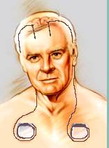
Figure 1.1. The mechanical device used to stimulate the brain has three implantable components: lead, extension and neurostimulator. [UMM01]
The procedure is not yet commonplace but is gaining popularity. There are currently 14,000 patients with deep brain stimulation devices implanted.
Surgery is performed through a hole in the skull about the size of a quarter. A microelectrode guided by a micro driver is passed through into the brain. The microelectrode measures the neural signals and can be used to find the exact location of the target.
The electrodes must be placed precisely in the right area in the brain in order to have a desired effect.
Signals picked up from the microelectrode are displayed on a computer monitor and as audio signals. Analysis of electrode recordings allows for a high degree of precision for stimulator placement. Once the appropriate structure is found, the microelectrode is replaced with a permanent electrode.
The patient is awake during the surgery to allow the surgical team to assess the patients brain function. While the electrode is being advanced, the patient does not feel any pain because of the brains unique nature and its inability to generate pain signals due to an absence of nociceptors or pain receptors. A local anesthetic is administered when the surgeon makes the opening in the skull. [Ahn03]
After the patient is diagnosed to require a DBS operation, the procedure of the operation is presented briefly below:
The patient is scanned with a magnetic resonance (MR) or a computed tomography (CT) scanner or both. This results in a series of MR and CT image slices. Usually both image types are used, since each technique has advantages and disadvantages over the other. For example anatomical structures on MR images can be seen more clearly, but there are slight deformations due to this technique and it is more noisy then CT images. CT images on the other hand are very accurate, but anatomical structures are not so visible like on MR images.
In order to take into account the advantages from both image types the image volumes composed of these two types of image slices are merged together. This process is called image fusion. To accurately fuse two images and volumes in 3D, a software application needs to find, recognize and match anatomical structures from the brain in each volume and try to deform one volume to match the other one. This technique is called registration.
After image fusion, when an accurate volume with good visibility is acquired the doctor needs to localize in it the target. This process is called targeting. In the end of the targeting process the coordinates and orientation of a trajectory pointing to a target point are received from the software application.
Targeting can be of two types:
Direct or absolute targeting, when the desired structure is visible on the digitally processed volume, and can be visually localized.
Indirect or relative targeting, when the desired structure is not visible at all, or not visible enough due to the limitations of the image acquisition devices. In this case the target is computed numerically by giving the position and orientation of the target relative to a visible structure, which visually can be localized.
After the surgeon analyzed the patient with the medical application, localized the target and found the optimal trajectory of the electrode the proper deep brain stimulation operation begins:
The stereotactic frame is positioned on the patients head. The stereotactic plane looks like a crown and it has certain freedoms of movement.
The doctor directs the drive onto the target, as the software computed the parameters. The drive is a mechanical gadget on the stereotactic frame, which drives the electrode and is controlled by a computer. It includes an electrical motor and the controller for the motor.
After that follows the electrophysiological exploration of the surroundings of the target. With a sensor electrode a device captures the electric signals from the brain. This signal is then amplified and processed with a software tool and visualized. The goal of this step is to localize accurately the desired structure by receiving feedback from the patient. In this step the sensor electrode is moved a little at a time toward the target point.
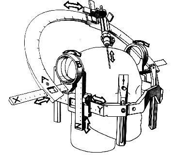
Fig 1.2. Schematic drawing of the arch of the Leksell stereotactic frame shows the two angles, A and B. [Dormont97]
The sensor electrode is a tube, with an isolated and very sharp wire at the end, usually around 4-10m s in diameter. It makes electrochemical contract with the ions of the neurons and is able to capture voltages of maximum 100V, which is then amplified about 10000 times. This way the signal coming from a neuron can be distinguished from the rest of the noise, which are due to the other small electronic signals from surrounding structures in the brain.
When the desired location is found it is stimulated with the same electrode. The sensor electrode produces an electric current and feedback. The current is amplified step by step and feedback is received from the patient. When the desired result is achieved on the patient, that is the stimulation position and current intensity is optimal for the patient to feel well, this phase ends.
The main goal of the medical imaging application DicomTools is to provide the targeting information. Without this the doctor can only approximate visually the target based on the image slices.
With targeting, the trajectory and penetration point of the stimulating electrode can be determined more accurately.
Like most of the real life practical applications, this application too involves many scientific areas.
DicomTools uses a mixture of knowledge from visualization techniques, image processing, object oriented programming and some anatomy knowledge.
Image processing is required to segment, recognize, reconstruct and manage anatomical structures of the human brain.
Visualization is required to make the segmented and recognized structures visible on a computer screen in order to simulate reality as well as possible.
Object oriented programming concepts were used to design the robust, safe and reusable components of the application.
Chapter 1 Introduction synthesized what is this paper about, what is deep brain stimulation, why there is a need for this type of medical visualization application and in what scientific domains does the application fit in.
This paper will present in the following chapters the details of the medical imaging and visualization application DicomTools.
In Chapter 2 Bibliography Outline the most important references to other papers are presented and where to find additional documentation on the issues presented here.
Chapter 3 Theoretical Background presents all the methods, best practices, theories, algorithms and other scientific knowledge which was used in order to implement DicomTools. It presents these theories from each scientific area: object oriented analysis and design concepts, visualization algorithms and common 3D mathematics and image processing, which at the time of writing this paper is an active field of research.
In Chapter 4 Project Specification and Architecture all the requirements and use cases for the medical application are listed. It can be considered as the vision document of the application. The requirements fall into four major categories: image file management, visualization in 2D and in 3D, image processing and targeting.
In Chapter 5 Analysis, Design and Implementation all the details for designing and implementing DicomTools are presented.
Chapter 6 Testing and Experimental Results will present the results obtained using this application. It will demonstrate how image files are read, anatomical structures segmented and how three dimensional models are reconstructed and visualized with DicomTools.
Chapter 7 User Guide will list the software and hardware requirements for running the application.
Chapter 8 Conclusions and Future Development will summarize the contribution of the author to writing this application and will outline what are the next development steps in the future regarding the development of this application.
Deep Brain Stimulation
In the following papers you can read detailed information and examples about the deep brain stimulation operation. The section 1.1 was written based on these papers.
[Ahn03] Ahn, Albert; Amin, Najma; Hopkins, Peter; Kelman, Alice; Rahman, Adeeb; Yang, Paul; Deep Brain Stimulation, 2003, https://biomed.brown.edu/Courses/BI108/BI108_2003_Groups/Deep_Brain_Stimulation/default.html
[Holloway05] Holloway, Kathryn; M.D., Deep Brain Stimulation, 2005, https://www1.va.gov/netsix-padrecc/page.cfm?pg=1
[UMM01] The University of Maryland Medical System Corporation, Departments of Neurology and Neurosurgery, Deep Brain Stimulation, 2001, https://www.umm.edu/neurosciences/deep_brain.html
[Dormont97] Didier Dormont, Philippe Cornu, Bernard Pidoux, Anne-Marie Bonnet, Alessandra Biondi, Catherine Oppenheim, Dominique Hasboun, Philippe Damier, Elisabeth Cuchet, Jacques Philippon, Yves Agid, and Claude Marsault , Chronic Thalamic Stimulation with Three-dimensional MR Stereotactic Guidance, AJNR Am J Neuroradiol 18:10931107, June 1997
DICOM Specification
[NEMA00]
National Electrical Manufacturers Association; Digital Imaging and
Communications in Medicine (DICOM);
This paper describes in detail the specification of the DICOM (Digital Imaging and Communications in Medicine) file format. It is the description of the DICOM 3 standard and it was used heavily during the development of the DicomFile library of DicomTools.
Visualization
[Lingrand02] Lingrand, Diane; Charnoz, Arnaud; Gervaise, Raphael; Richard, Karen; The Marching Cubes, 2002, https://www.essi.fr/~lingrand/MarchingCubes/accueil.html
[Lorensen87] Lorensen, William E.; Cline, Harvey E.; Marching Cubes: A High Resolution 3D Surface Construction Algorithm, General Electric Company, Corporate Research and Development, Schenectady, New York 12301, 1987, https://www.fi.muni.cz/~sochor/PA010/Clanky/2/p163-lorensen.pdf
The above two papers describe in detail the Marching Cubes algorithm which is heavily used in DicomTools. The first paper is an overview of the algorithm and the second is the original paper written by the author and explores in grater depth this algorithm. Readers should keep in mind that the Marching Cubes algorithm is patented and for commercial use license is required from the authors.
[Schroeder] Schroeder, William J.; Zarge, Jonathan A.; Lorensen, William E.; Decimation of Triangle Meshes, General Electric Company, Schenectady, New York, https://www.dgm.informatik.tu-darmstadt.de/courses/cg2/cg2_ex3.pdf
This paper describes in details the decimation algorithm used in DicomTools to reduce the sizes of the polygonal mesh models and it is presented in paragraph 3.3.3 Mesh Decimation.
[VTK04] Kitware Inc, VTK 4.5.0 Documentation, 2004, https://www.vtk.org
The technical information from VTK website was used in several parts of this paper to demonstrate and exemplify the usage of the Visualization ToolKit. They are taken mostly from the VTK documentation, which is downloadable from VTKs website, the Frequently Asked Questions section, and the VTK overview.
Also the next two papers are also from VTKs website, but we emphasize it separately because it contains a very compact and useful overview of VTK.
[Schroeder04a], William J.; VTK An Open Source Visualization Toolkit, Kitware, 2000, https://gd.tuwien.ac.at/visual/public.kitware.com/vtk/doc/presentations/vde2000.ppt
[Schroeder04b], William J.; The Visualization Toolkit An Overview, Kitware Inc; https://gd.tuwien.ac.at/visual/public.kitware.com/vtk/doc/presentations/VTKOverview.ppt
Image Processing
[Ibanez05] Ibanez, Luis; Schroeder, Will;
This paper describes in details the usage of ITK (the Insight Segmentation and Registration ToolKit) and it was used many times during the development of the application. Also the section 3.4 of chapter 3 is based upon this book.
[ITK05] Kitware Inc, Insight Segmentation and Registration Toolkit, https://www.itk.org
This is the ITKs website and it includes the ITK source code, binaries and documentation for different ITK versions. It was used to exemplify the filters used in DicomTools.
In order to design such a large and complex medical visualization application as DicomTools there were used a couple of best practices and design patterns from the object oriented programming domain.
For implementing the entire requirements besides medical and biological knowledge one must also have 3D mathematics, visualization and image processing background. They will be presented in the following sections.
The following figure illustrates the elements of the application. In the diagram there are shown the main phases and sub phases of DicomTools. The following paragraphs of this chapter and the other chapters too will present in details the notions of a particular phase or stage of the application. The order of the phases is approximately also the same as in the diagram. It should be noted that this is not an UML diagram. The ellipses represents the main phases or states of the application while the rectangles represents sub phases or alternatives.
The first phase or ellipse Find Files refers to the state in which the user is prompted to select some image files on which the work will be carried out. This can be done in the form of a dialog window for opening files or directories or from the command prompt.
After files have been selected to work with, they should be rearranged into consistent sets from which consistent image volumes can be created. This is realized by grouping for instance DICOM files together in such a way the files from the same patient, same modality, same study and same image acquisition series number to be together. This information can be found in the header of DICOM files and will be read and compared to other files in this stage. After files have been grouped they are sorted after the position they would take in the image volume if it would be created. Finally duplicate files should be removed to prevent the malformation of the image volume, for example by reading a file twice. More about DICOM files one can read in the next paragraph The DICOM Standard.
When the desired files are arranged they are ready to be read. Reading the image files makes the pixel data be available in memory and to be able to undergo image processing. For converting image files into voxel data the file IO libraries of VTK and ITK were used since they are used heavily for image processing and visualization of the application. A special library for DICOM file manipulation was also created, from scratch, because this has more flexibility manipulating DICOM tags then the built-in VTK and ITK libraries. This library is used in the process of arranging image files. More about VTK, ITK, different file readers and methods of file input output one can read in chapter 5. Analysis, Design and Implementation.
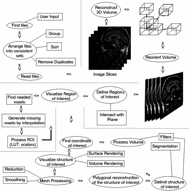
Figure 3.1. Organization chart of the application
The purpose of reading image files is to make available pixels in memory packed into objects which are useful for the programmer and permits further operations. This corresponds to the phase Reconstruct 3D Volume. This reconstruction is taken care of by VTK. VTK reads the pixels of every image file given as input and puts the pixel values into a linear scalar array. Scalars are accessed with logical (extent or i, j, k, integer number) coordinates. Since pixels in an image and voxels in a volume are placed at a certain distance from one another, that is they have a dimension, this information is also stored. In VTK each voxel has also a cell associated with it. The cells are usually rectangular parallelepipeds with their center at the physical (world) coordinates of the voxel values Cx, Cy, Cz and their extremities in the form: (-SpacingX/2 + Cx, +SpacingX/2 + Cx), (-SpacingY/2 + Cy, +SpacingY/2, Cy), (-SpacingZ/2 + Cz, +SpacingZ/2 + Cz). The point at the center has the same scalar value as the voxel value associated with that cell. Scalar values of points in the cell at other positions then the center are computed by interpolation taking into account neighbor cells.
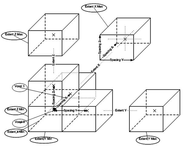
Figure 3.2. Cell structure of the reconstructed 3D volume.
Often image files are oriented in different ways relative to the patient. In order to simplify further computations it is desired to reorient newly constructed image volumes according to a chosen orientation. The destination coordinate system in which all the volumes will be reoriented is the Patient Coordinated System, defined in the DICOM Standard and presented in more details in paragraph 5.3. Implementation Challenges of chapter 5.
After reconstructing and reorienting an image volume it can be used for processing. Such a processing is required when we want to visualize the intersection of the volume with a plane. This again is realized by the class vtkImagePlaneWidget from VTK. It selects the voxels closest to the intersecting plane and applies texture mapping on the polygon which is the result of the intersection of the image volume with the plane. In order to fill the empty space between voxels interpolation is used. In VTK usually there are tree types of interpolations: nearest neighbor, linear and cubic. After the scalars of the texture are computed they can be mapped to color or intensity values. About other visualization methods one can read in paragraph 5 of this chapter Visualization Methods. About mapping scalar values to color values see paragraph 5.2.5. Visualization.
Visualization methods help the user to locate a point in the 3D volume. This process is called targeting. Usually such points of interest, also called targets, will be the destination point where a certain electrode must reach.
When a target is set, the structure in which lies and structures in the vicinity must be reconstructed. This is done by processing the image by applying different filters on it. One of the main goals is to delimit the structure of interest in which the target can be found. This is realized with segmentation. Details about segmentation methods will be presented in paragraph 6 of this chapter: Image Processing.
After the structure of interest is delimited its surface can be reconstructed. This is done with the algorithm Marching Cubes, presented later in this chapter.
The resulting mesh model is further processed in order to reduce its size. Reducing the size of a polygon mesh is done with a decimation algorithm. Other filters operating on polygonal data are also used to increase the quality of the decimated mesh model, for example smoothing.
Finally the delimited structure of interest can be visualized with a chosen method presented in this chapter or by combining more visualization methods. At this stage the Targeting-Segmentation-Visualization loop starts again. The goal of this loop is to enhance at each iteration the position of the target and the precision of the detected structures.
The Digital Imaging and Communications in Medicine (DICOM) is created by
the
The purpose of the DICOM standard is to be a:
hardware interface
a minimum set of software commands
consistent set of data formats
communication of digital image information
development and expansion of picture archiving and communication systems
interface with other systems of hospital information
creation of diagnostic information data bases
[NEMA00]
The DICOM Standard facilitates interoperability of devices claiming conformance. In particular, it:
Addresses the semantics of Commands and associated data. For devices to interact, there must be standards on how devices are expected to react to Commands and associated data, not just the information which is to be moved between devices;
Is explicit in defining the conformance requirements of implementations of the Standard. In particular, a conformance statement must specify enough information to determine the functions for which interoperability can be expected with another device claiming conformance.
Facilitates operation in a networked environment, without the requirement for Network Interface Units.
Is structured to accommodate the introduction of new services, thus facilitating support for future medical imaging applications.
Makes use of existing international standards wherever applicable, and itself conforms to established documentation guidelines for international standards.
The latest version of the DICOM specification is version 3.0.
A DICOM file consists of a set of data elements. Each data element has a tag or id, which consists of the group number and element number of the respective data element. The Value Representation Field (VR) specifies how the data in the value field should be interpreted. In the DICOM standard there are a few well defined value representation types. Some examples are: decimal string (DS), character sequence (CS), unique identifier (UI), etc.
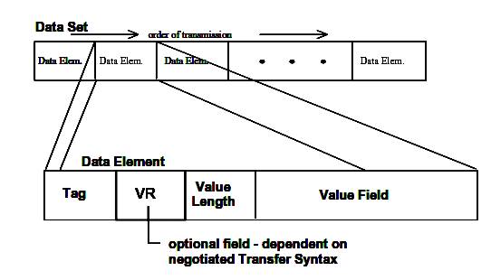
Figure 3.3. DICOM Dataset and Data Element structures.
Data Element Tag: An ordered pair of 16-bit unsigned integers representing the Group Number followed by Element Number.
Note: PS 3.x refers to the DICOM Specification 3, chapter x document downloadable from the internet.
Value Representation: A two-byte character string containing the VR of the Data Element. The VR for a given Data Element Tag shall be as defined by the Data Dictionary as specified in PS 3.6. The two characters VR shall be encoded using characters from the DICOM default character set.
Value Length:
- either a 16 or 32-bit (dependent on VR and whether VR is explicit or implicit) unsigned integer containing the Explicit Length of the Value Field as the number of bytes (even) that make up the Value. It does not include the length of the Data Element Tag, Value Representation, and Value Length Fields
- A 32-bit Length Field set to Undefined Length (FFFFFFFFH). Undefined Lengths may be used for Data Elements having the Value Representation (VR) Sequence of Items (SQ) and Unknown (UN). For Data Elements with Value Representation OW or OB Undefined Length may be used depending on the negotiated Transfer Syntax (see Section 10 and Annex A).
Note: =The decoder of a Data Set should support both Explicit and
Undefined Lengths for VRs of SQ and UN and, when applicable, for VRs of OW and
Value Field: An even number of bytes containing the Value(s) of the Data Element.
The data type of Value(s) stored in this field is specified by the Data Element's VR. The VR for a given Data Element Tag can be determined using the Data Dictionary in PS 3.6, or using the VR Field if it is contained explicitly within the Data Element. The VR of Standard Data Elements shall agree with those specified in the Data Dictionary.
The Value Multiplicity specifies how many Values with this VR can be placed in the Value Field. If the VM is greater than one, multiple values shall be delimited within the Value Field as defined previously. The VMs of Standard Data Elements are specified in the Data Dictionary in PS 3.6.
Value Fields with Undefined Length are delimited through the use of Sequence Delimitation Items and Item Delimitation Data Elements.
[NEMA00]
The application is written entirely in C++ and it is object oriented. Therefore the design and implementation of the application is based on the known object oriented analysis and design processes, for example the Rational Unified Process.
For common and repetitive problems and tasks design patterns were used. Design patterns make it easier to reuse successful designs and architectures. Expressing proven techniques as design patterns makes them more accessible to developers of new systems. Design patterns help you choose design alternatives that make a system reusable and avoid alternatives that compromise reusability. Design patterns can even improve the documentation and maintenance of existing systems by furnishing an explicit specification of class and object interactions and their underlying intent. Put simply, design patterns help a designer get a design 'right' faster. [Gamma04]
When mesh-models are initially created, they are usually formed around a specific location (typically the origin) and they usually have a particular size and orientation. This occurs because we are using simplified algorithms which make calculations and understanding easier. However, for the final scene, the models need to be moved, scaled and rotated into their final positions.
These changes can be achieved by applying an affine transformation matrix to the vertices of the polygon mesh. These transformations are implemented by multiplying the appropriate vertex by a matrix.
Often in the application there were several places where we needed to transform a point or a vector from one coordinate system to another.
For example the space of voxels with its coordinate system having the origin in one corner of the parallelepiped representing the voxels and with the axes of the coordinate system being the edges of this parallelepiped starting from the origin is a good coordinate system for image processing algorithms that operate on the entire medical volume.
On the other hand some brain structures are reported to have a certain location and orientation relative to other structures. For the doctor is easier to work in a relative coordinate system inside the patients brain.
Therefore coordinate transformations from one coordinate system into another is a very common task in DicomTools.
Below are presented some of the basic transformations in space.
To scale a mesh (stretch along x-axis) we apply the following to each point:
In this case, x component of each point has been multiplied by s.
This scaling matrix can be generalized as
where sx, sy and sz are scaling factors along the x-axis, y-axis and z-axis respectively.
To rotate a point ![]() degrees
about the z-axis, we multiply the point by the following matrix:
degrees
about the z-axis, we multiply the point by the following matrix:
For rotations about the x-axis and y-axis, we apply the following:
In order to translate a point we can add a vector to it:
![]()
Scaling and rotation are performed by matrix multiplication, and
translation is performed by vector addition. It would be simplify matters if we
could also apply translation by matrix multiplication. Vector addition can be
simulated by multiplication by using Homogeneous co-ordinates.
To convert a vertex to Homogeneous co-ordinates, we simply add a ![]() co-ordinate,
with a value one:
co-ordinate,
with a value one:
![]()
To convert a matrix to homogeneous co-ordinates we add an extra row and an extra column:
Using the homogeneous matrix, translation can be implemented by matrix multiplication:
[Power04]
Representing 3D image volumes composed of a set of voxels on a 2D computer screen composed of pixels is not a trivial task.
For visualizing in 3D there are more alternatives. In the following paragraphs the different alternatives for visualizing a 3D volume will be presented. However this list of visualization techniques is not complete. There are other several techniques for visualization and they may cross the boundaries of these standard visualization methods by combining more of these methods into on technique.
A possibility for visualizing 3D objects is surface rendering. This section briefly describes a general set of 3D scalar and vector surface rendering techniques. The first four descriptions deal with scalar field techniques and the other two with vector field techniques.
Scalar glyphs is a technique which puts a sphere or a diamond on every data point. The scale of the sphere or diamond is determined by the data value. The scalar glyphs may be colored according to the same scalar field or according to another scalar field. In this way correlations can be found. As no interpolations are needed for this technique it consumes few CPU seconds.
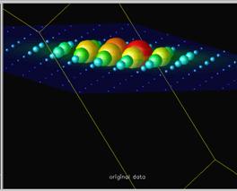
Figure 3.4. Image from IBM Visualization Data Explorer [Grinstein96]
This technique produces surfaces in the domain of the scalar quantity on which the scalar quantity has the same value, the so-called isosurface value. The surfaces can be colored according to the isosurface value or they can be colored according to another scalar field using the texture technique. The latter case allows for the search for correlation between different scalar quantities.
There are different methods to generate the surfaces from a discrete set of data points. All methods use interpolation to construct a continuous function. The correctness of the generated surfaces depends on how well the constructed continuous function matches the underlying continuous function representing the discrete data set.
The method which is used in the software application is known as the Marching Cube Algorithm.
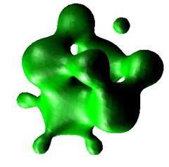
Figure 3.5. Isosurface - function x^2+y^2+z^2+sin(4.0*x)+sin(4.0*y)+sin(4.0*z)=1.0 [Boccio05]
This technique makes it possible to view scalar data on a cross-section of the data volume with a cutting plane. One defines a regular, Cartesian grid on the plane and the data values on this grid are found by interpolation of the original data. A convenient color map is used to make the data visible.
Figure 3.6. Example for cutting planes [Strand7]
It often occurs that one wants to focus on the influence of only two independent variables (i.e. coordinates). Thus, the other independent variables are kept constant. This is what the orthogonal slicer method does. For example, if the data is defined in spherical coordinates and one wants to focus on the angular dependences for a specific radius, the orthogonal slicer method constructs the corresponding sphere. No interpolation is used since the original grid with the corresponding data is inherited. A convenient color map is used to make the data visible.
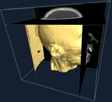
Figure 3.7. Example for orthogonal slicers. [Guatam05]
This technique uses needle or arrow glyphs to represent vectors at each data point. The direction of the glyph corresponds to the direction of the vector and its magnitude corresponds to the magnitude of the vector. The glyphs can be colored according to a scalar field.
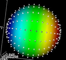
Figure 3.8. Glyphs representing the orientations of normals on a sphere in a VTK application
This is a set of methods for outlining the topology, i.e. the field lines, of a vector field. Generally, one takes a set of starting points, finds the vectors at these points by interpolation, if necessary, and integrates the points along the direction of the vector. At the new positions the vector values are found by interpolation and one integrates again. This process stops if a predetermined number of integration steps have been reached or if the points end up outside the data volume. The calculated points are connected by lines.
The difference between streak lines and streak lines is that the streamlines technique considers the vector field to be static whereas the streak lines technique considers the vector field to be time dependent. Hence, the streak line technique interpolates not only in the spatial direction, but also in the time direction. The particle advection method places little spheres at the starting points representing mass less particles. The particles are also integrated along the field lines. After every integration step each particle is drawn together with a line or ribbon tail indicating the direction in which the particle is moving.
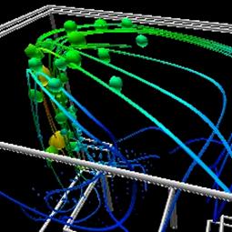
Figure 3.9. Here the spherical glyphs represent particle advection of heated air around a room. The streamlines show the complete particle flow in the enclosed space. Color mapping is also used to represent the temperature of particles at specific points. [UoB]
This is a technique to color arbitrary surfaces, e.g. those generated by the isosurface techniques, according to a 3D scalar field. An interpolation scheme is used to determine the values of the scalar field on the surface. A color map is used to assign the color. [SciViz]
In order to visualize a structure from within a set of voxels the delimiting surface of the object is reconstructed and visualized. Such an algorithm which delimits an isosurface from within a volume is presented below.
Marching cubes is one of the latest algorithms of surface construction used for viewing 3D data. In 1987 Lorensen and Cline (GE) described the marching cubes algorithm. This algorithm produces a triangle mesh by computing isosurfaces from discrete data. By connecting the patches from all cubes on the isosurface boundary, we get a surface representation.
The marching cubes algorithm creates triangle models of constant density surfaces from 3D medical data. Using a divide-and-conquer approach to generate inter-slice connectivity, we create a case table that defines triangle topology. The algorithm processes the 3D medical data in scan-line order and calculates triangle vertices using linear interpolation. We find the gradient of the original data, normalize it, and use it as a basis for shading the models. The detail in images produced from the generated surface models is the result of maintaining the inter-slice connectivity, surface data, and gradient information present in the original 3D data. [Lorensen87]
In order to explain this technique, we are going to introduce the marching squares algorithm which uses the same approach in 2D. After having presented some marching squares ambiguous cases we will be able to describe the marching cubes algorithm and an ambiguous case resolution.
The marching squares algorithm aims at drawing lines between interpolated values along the edges of a square, considering given weights of the corners and a reference value. Let's consider a 2D grid as shown in the next picture.
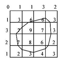
Figure 3.10. The marching square algorithm example.
Each point of this grid has a weight and here the reference value is
known as 5. To draw the curve whose value is constant and equals the reference
one, different kinds of interpolation can be used. The most used is the linear
interpolation.
In order to display this curve, different methods can be used. One of them
consists in considering individually each square of the grid. This is the
marching square method. For this method 16 configurations have been enumerated,
which allows the representation of all kinds of lines in 2D space.
Figure 3.11. The marching squares algorithm cases.
While trying this algorithm on different configurations we realize that some cases may be ambiguous. That is the situation for the squares 5 and 10.
Figure 3.12. The marching squares ambiguous cases.
As you can see on the previous picture we are not able to take a decision on the interpretation of this kind of situation. However, these exceptions do not imply any real error because the edges keep closed.
Following the marching squares algorithm we can adapt our approach to the 3D case: this is the marching cubes algorithm. In a 3D space we enumerate 256 different situations for the marching cubes representation. All these cases can be generalized in 15 families by rotations and symmetries:
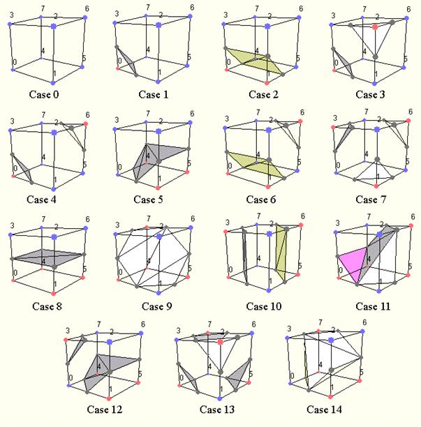
Figure 3.13. The cases of the marching cubes algorithm.
In order to be able to determine each real case, a notation has been adopted. It aims at referring each case by an index created from a binary interpretation of the corner weights.
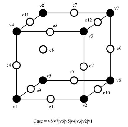
Figure 3.14. Notation of the marching cubes cases.
In this way, vertices from 1 to 8 are weighted from 1 to 128 (v1 = 1, v2 = 2, v3 = 4, etc.); for example, the family case 3 example you can see in the picture above, corresponds to the number 5 (v1 and v3 are positive, 1 + 4 = 5).
To all this cubes we can attribute a complementary one. Building a complementary cube consists in reversing normals of the original cube. In the next picture you can see some instances of cubes with their normals.
Figure 3.15. Complementary cubes.
The creation of these complementary cubes allows us to give an orientation to the surface.
As for the marching squares we meet some ambiguous marching cubes cases: for the family 4 and 10. But in 3D space a solution has to be found because of the topology problems these situations create. However not only real ambiguous cases can create topology disfunctions, some classical families are incompatible. See for instance the next picture.
To cope with these topology errors (as holes in the 3D model), 6 families have been added to the marching cubes cases. These families have to be used as complementary cases. For instance, in the previous picture, you have to use the case 6c instead of the standard complementary of the case 6.
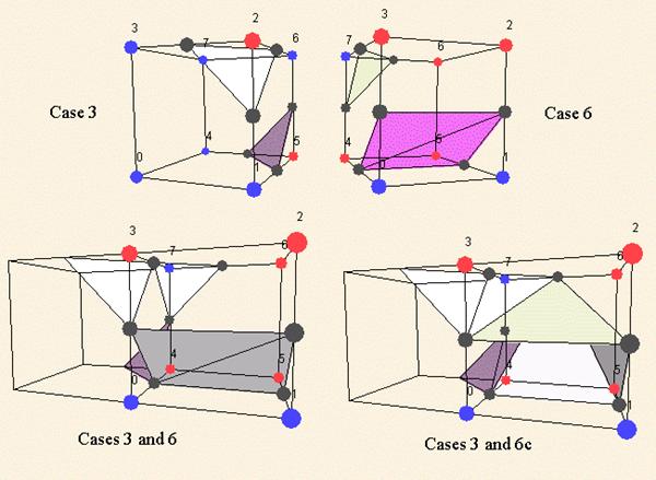
Figure 3.16. Marching cubes ambiguous cases.
Figure 3.17. Marching cubes complementary cases. [Lingrand02]
After the resulting surface is generated it will represented by polygons. To enhance the quality of the resulting polygonal mesh several filters may be applied. Such a filter is the decimation of triangle meshes.
Triangle mesh decimation is an algorithm to reduce the number of triangles in a triangle mesh. The objective of mesh decimation is to reduce the memory size needed for the representation of an object with good approximation of the original object. This reduction, as the name suggests, can be from 10 to 50 times or even more. This yields not only less memory usage for the representation of the mesh but also faster processing.
The algorithm proceeds as follows. Each vertex in the triangle list is evaluated for local planarity (i.e., the triangles using the vertex are gathered and compared to an 'average' plane). If the region is locally planar, that is if the target vertex is within a certain distance of the average plane (i.e., the error), and there are no edges radiating from the vertex that have a dihedral angle greater than a user-specified edge angle (i.e., feature angle), and topology is not altered, then that vertex is deleted. The resulting hole is then patched by re-triangulation. The process continues over the entire vertex list (this constitutes an iteration). Iterations proceed until a target reduction is reached or a maximum iteration count is exceeded. [VTK04]
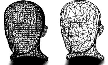
Figure 3.18. Mesh model before (left) and after decimation (right). [SMS02]
Polygon mesh models are distinguished by the fact that the model only approximates the actual objects represented. A Shading model must apply some reflection model (e.g. Phong reflection) to these faces, in order to determine how the face is to be colored. The reflection model should take into account orientation of light sources, position of viewer and properties of the surface being rendered. Polygon meshes are typically collections of planer faces, which model smooth surfaces. Combining diffuse and specular reflection models, we get the following model for light intensity at a point on a surface (the underlined term must be repeated for each additional light source in the scene);
![]()
The possibilities for shading the surface of a 3D object represented by a polygonal mesh are presented below.
A naive Flat Shading technique will apply a refection model to one point on a face and the shade determined is applied to the entire face. This method is quick and produces acceptable results if smooth surfaces are not involved. Specular reflection will be shown in flat shading, but only very coarsely. If realistic scenes are to be generated, flat shading requires so many polygons as to be infeasible. Regardless of the number of polygons, flat shading will almost always give a faceted appearance in certain areas because of Mach Banding, which tends to exaggerate the differences between faces. Flat shading is generally only used for prototyping or testing an application where speed, not accuracy is important. Other methods can produce more realistic displays with much fewer polygons.
Figure 3.19: Shading methods (left to right); Flat shading, Smooth shading no specular, Smooth shading f=20, Smooth shading f=200.
In order to accurately render curved surfaces represented by a polygon mesh, we need to implement an Incremental or Smooth Shading technique to smooth out the faceted nature of the mesh. The first smooth shading technique developed was Gouraud Shading.
This method simply calculates the Surface Normal at each vertex by averaging the normals of the faces which share the vertex.
Figure 3.20. Averaging Normals.
This average normal will coincide closely with the normal of the actual modeled surface at that point. This vector is then used in a reflection model to determine the light intensity at that point. This process is repeated for all vertices in the model. Once the correct intensity has been calculated for each vertex, these are used to interpolate intensity values over the face. The interpolation scheme is known as bi-linear interpolation.

Figure 3.21. Interpolating Intensities.
Intensities are known for![]() ,
,![]() and
and![]() .
.
![]() and
and ![]() can
be interpolated as follows:
can
be interpolated as follows:
Gouraud smoothes the faceted appearance of meshes, because the interpolated intensities along an edge are used to shade both polygons which share that edge. This means that there is not a discontinuity of color at the edges of adjoining faces.
However, although the mesh appears smooth, the polygons are still visible at the edge of the object when viewed as a silhouette. Gouraud can also interpolate incorrectly which results in some rendering errors which remove some detail (figure 7.15).

Figure 3.22. Surface Rendered Incorrectly.
The biggest problem with Gouraud shading is the fact it reproduces specular shading poorly and if specular reflection is displayed, it is determined by the polygon mesh rather than the modeled surface. If a highlight occurs in the middle of a polygon, but not at any of the vertices, the highlight will not be rendered by interpolation. Also, Mach banding can occur when specular refection is incorporated into Gouraud, for this reason, the specular component is often ignored when using Gouraud, giving 'smother' results.

Figure 3.23. Specular Reflection Not Rendered.
Phong shading overcomes the problems of specular reflection encountered in Gouraud shading. This method again calculates the normals at the vertices by averaging the normals for the faces at that vertex. These vertex normals are then interpolated across the face.

Figure 3.24. Interpolating Normals.
Thus we have a good approximation of the surface normal at each scan line position (pixel) and therefore we are able to calculate more accurately the intensity at that point, including specular highlights. The interpolation scheme for normals is similar to Intensity interpolation.

Figure 3.25. Bi-Linear
![]()
![]()
Phong shading requires intensity calculations at each point on the face, so is therefore far more expensive that Gouraud which only performs intensity calculations at the vertices. Note that the computation of normals in both Gouraud and Phong must be done in world coordinates, as pre-warping distorts the relative orientation between surface, light-source and eye. Both these methods can be integrated with Z-Buffer or scan line filling algorithms [Power04]
Volume rendering is a term used to describe a rendering process applied to 3D data where information exists throughout a 3D space instead of simply on 2D surfaces defined in 3D space. There is not a clear dividing line between volume rendering and geometric techniques. [Schroeder02]
Volume rendering is a technique for visualizing sampled functions of three spatial dimensions by computing 2-D projections of a colored semitransparent volume. This is usually done by the Ray Casting algorithm.
The basic goal of ray casting is to allow the best use of the three-dimensional data and not attempt to impose any geometric structure on it. It solves one of the most important limitations of surface extraction techniques, namely the way in which they display a projection of a thin shell in the acquisition space. Surface extraction techniques fail to take into account that, particularly in medical imaging, data may originate from fluid and other materials which may be partially transparent and should be modeled as such. Ray casting doesn't suffer from this limitation.
Currently, most volume rendering that uses ray casting is based on the Blinn/Kajiya model. In this model we have a volume which has a density D(x,y,z), penetrated by a ray R.
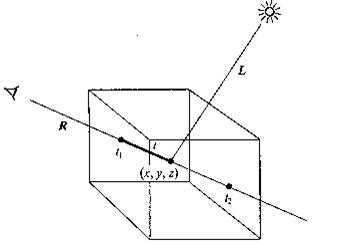
Figure 3.26. A ray R cast into a scalar function of three spatial variables.
At each point along the ray there is an illumination I(x,y,z) reaching the point (x,y,z) from the light source(s). The intensity scattered along the ray to the eye depends on this value, a reflection function or phase function P, and the local density D(x,y,z). The dependence on density expresses the fact that a few bright particles will scatter less light in the eye direction than a number of dimmer particles. The density function is parameterized along the ray as:
D(x(t), y(t), z(t)) = D(t)
The illumination from the source as:
I(x(t), y(t), z(t)) = I(t)
and the illumination scattered along R from a point distance t along the ray is:
I(t)D(t)P(cos )
where is the angle between R and L, the light vector, from the point of interest.
Determining I(t) is not trivial - it involves computing how the radiation from the light sources is attenuated and/or shadowed due to its passing through the volume to the point of interest. This calculation is the same as the computation of how the light scattered at point (x,y,z) is affected in its journey along R to the eye. In most algorithms, however, this calculation is ignored and I(x,y,z) is set to be uniform throughout the volume.
For most practical applications we're interested in visualization, and including the line integral from a point (x,y,z) to the light source may actually be undesirable. In medical imaging, for example, it would be impossible to see into areas surrounded by bone if the bone were considered dense enough to shadow light. On the other hand, in applications where internal shadows are desired, this integral has to be computed.
The attenuation due to the density function along a ray can be calculated as:
where ![]() is a
constant that converts density to attenuation.
is a
constant that converts density to attenuation.
The intensity of the light arriving at the eye along direction R due to all the elements along the ray is given by:
[Pawasauskas97]
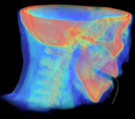
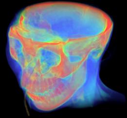
Figure 3.27. Examples for Volume Rendering taken from Kitwares VolView 2.0
In order to realize the visualization of a structure from a 3D volume or of the volume itself several image processing algorithms were used.
Histogram equalization is the process of redistributing uniformly the colors or intensities of a color palette among the pixels of a dataset. This results in a better visual representation of an image, since every color is used thus revealing more detail in the image with the normalized histogram. Particular cases of histogram equalization are histogram stretching and histogram shrinking.
For equalizing the histogram of a volume the algorithm Histogram Equalization by Pair wise Clustering was used. It uses a local error optimization strategy to generate near optimal quantization levels. The algorithm is simple to implement and produces results that are superior then those of other popular image quantization algorithms. [Velho]
This algorithm was adapted to grey scale images.
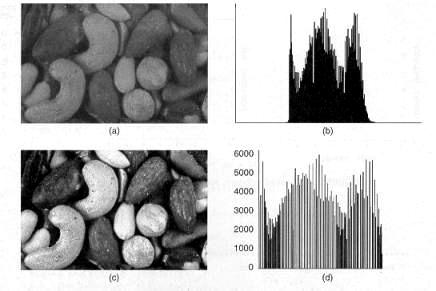
Figure 3.28. (a) Original image; (b) Histogram of original image; (c) Equalized image; (d) Histogram of equalized image. [Luong]
In many cases it is much better to preprocess or post process an image with a certain filter, because this way the quality of the image can be increased. Some of these filters include noise removal filters, like the edge preserving Gaussian Smooth filter, filters used on binary images like eroding and closing. For more details see [Fisher94].
Segmentation is the method of delimiting a region inside of an image. This is done by unifying pixels into regions based on a certain criteria. After every pixel is classified into a region the final image will be composed of these regions called segments.
Segmentation of medical images is a challenging task. A myriad of different methods have been proposed and implemented in recent years. In spite of the huge effort invested in this problem, there is no single approach that can generally solve the problem of segmentation for the large variety of image modalities existing today.
The most effective segmentation algorithms are obtained by carefully customizing combinations of components. The parameters of these components are tuned for the characteristics of the image modality used as input and the features of the anatomical structure to be segmented. [Ibanez05]
Region growing algorithms have proven to be an effective approach for image segmentation.
The basic approach of a region growing algorithm is to start from a seed region (typically one or more pixels) that are considered to be inside the object to be segmented. The pixels neighboring this region are evaluated to determine if they should also be considered part of the object. If so, they are added to the region and the process continues as long as new pixels are added to the region. Region growing algorithms vary depending on the criteria used to decide whether a pixel should be included in the region or not, the type connectivity used to determine neighbors, and the strategy used to visit neighboring pixels.

Figure 3.29. Example for region growing. [Marshall97]
Watershed segmentation classifies pixels into regions using gradient descent on image features and analysis of weak points along region boundaries. Imagine water raining onto a landscape topology and flowing with gravity to collect in low basins. The size of those basins will grow with increasing amounts of precipitation until they spill into one another, causing small basins to merge together into larger basins. Regions (catchment basins) are formed by using local geometric structure to associate points in the image domain with local extrema in some feature measurement such as curvature or gradient magnitude. This technique is less sensitive to user-defined thresholds than classic region-growing methods, and may be better suited for fusing different types of features from different data sets. The watersheds technique is also more flexible in that it does not produce a single image segmentation, but rather a hierarchy of segmentations from which a single region or set of regions can be extracted a-priori, using a threshold, or interactively, with the help of a graphical user interface.
The strategy of watershed segmentation is to treat an image f as a height function, i.e., the surface formed by graphing f as a function of its independent parameters, 1x RU. The image f is often not the original input data, but is derived from that data through some filtering, graded (or fuzzy) feature extraction, or fusion of feature maps from different sources. The assumption is that higher values of f (or -f) indicate the presence of boundaries in the original data.
Watersheds may therefore be considered as a final or intermediate step in a hybrid segmentation method, where the initial segmentation is the generation of the edge feature map.
Gradient descent associates regions with local minima of f (clearly interior points) using the watersheds of the graph of f, as in Figure 3.27. That is, a segment consists of all points in U whose paths of steepest descent on the graph of f terminate at the same minimum in f.
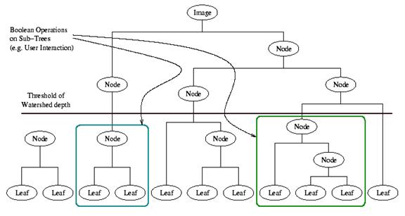 Figure 3.30. A
watershed segmentation combined with a saliency measure (watershed depth)
produces a hierarchy of regions. Structures can be derived from images by
either thresholding the saliency measure or combining sub trees within the
hierarchy.
Figure 3.30. A
watershed segmentation combined with a saliency measure (watershed depth)
produces a hierarchy of regions. Structures can be derived from images by
either thresholding the saliency measure or combining sub trees within the
hierarchy.
Thus, there are as many segments in an image as there are minima in f. The segment boundaries are ridges in the graph of f. In the 1D case, the watershed boundaries are the local maxima of f and the results of the watershed segmentation is trivial. For higher dimensional image domains, the watershed boundaries are not simply local phenomena; they depend on the shape of the entire watershed.
The drawback of watershed segmentation is that it produces a region for each local minimum - in practice too many regions - and an over segmentation results. To alleviate this, we can establish a minimum watershed depth. The watershed depth is the difference in height between the watershed minimum and the lowest boundary point. In other words, it is the maximum depth of water a region could hold without flowing into any of its neighbors. Thus, a watershed segmentation algorithm can sequentially combine watersheds whose depths fall below the minimum until all of the watersheds are of sufficient depth. This depth measurement can be combined with other saliency measurements, such as size. The result is a segmentation containing regions whose boundaries and size are significant. Because the merging process is sequential, it produces a hierarchy of regions. Previous work has shown the benefit of a user-assisted approach that provides a graphical interface to this hierarchy, so that a technician can quickly move from the small regions that lie within an area of interest to the union of regions that correspond to the anatomical structure.
The paradigm of the level set is that it is a numerical method for tracking the evolution of contours and surfaces.
Instead of manipulating the contour directly, the contour is embedded as the zero level set of a higher dimensional function called the level-set function, y(X, t). The level-set function is then evolved under the control of a differential equation. At any time, the evolving contour can be obtained by extracting the zero level-set G((X), t) = from the output.
The main advantages of using level sets is that arbitrarily complex shapes can be modeled and topological changes such as merging and splitting are handled implicitly.
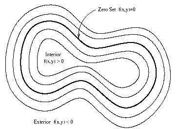
Figure 3.31. Concept of zero set in a level set.
Level sets can be used for image segmentation by using image-based features such as mean intensity, gradient and edges in the governing differential equation. In a typical approach, a contour is initialized by a user and is then evolved until it fits the form of an anatomical structure in the image. Many different implementations and variants of this basic concept have been published in the literature.
The remainder of this section introduces practical examples of some of the level set segmentation methods available in ITK. Understanding these features will aid in using the filters more effectively.
Each filter makes use of a generic level-set equation to compute the update to the solution y of the partial differential equation
![]()
where A is an advection term, P is a propagation (expansion) term, and Z is a spatial modifier term for the mean curvature k
The scalar constants a b, and g weight the relative influence of each of the terms on the movement of the interface. A segmentation filter may use all of these terms in its calculations, or it may omit one or more terms. If a term is left out of the equation, then setting the corresponding scalar constant weighting will have no effect. All of the level-set based segmentation filters must operate with floating point precision to produce valid results.
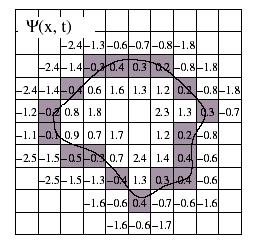
Figure 3.32. The implicit level set surface G is the black line superimposed over the image grid. The location of the surface is interpolated by the image pixel values. The grid pixels closest to the implicit surface are shown in gray.
The third, optional template parameter is the numerical type used for calculations and as the output image pixel type. The numerical type is float by default, but can be changed to double for extra precision. A user-defined, signed floating point type that defines all of the necessary arithmetic operators and has sufficient precision is also a valid choice. You should not use types such as int or unsigned char for the numerical parameter. If the input image pixel types do not match the numerical type, those inputs will be cast to an image of appropriate type when the filter is executed.
Most filters require two images as input, an initial model y(X, t) = 0, and a feature image, which is either the image you wish to segment or some preprocessed version. You must specify the isovalue that represents the surface G in your initial model. The single image output of each filter is the function y at the final time step. It is important to note that the contour representing the surface G is the zero level-set of the output image, and not the isovalue you specified for the initial model. To represent G using the original isovalue, simply add that value back to the output.
The solution G is calculated to sub pixel precision. The best discrete approximation of the surface is therefore the set of grid positions closest to the zero-crossings in the image.
The itk::ZeroCrossingImageFilter operates by finding exactly those grid positions and can be used to extract the surface.
There are two important considerations when analyzing the processing time for any particular level-set segmentation task: the surface area of the evolving interface and the total distance that the surface must travel. Because the level-set equations are usually solved only at pixels near the surface (fast marching methods are an exception), the time taken at each iteration depends on the number of points on the surface. This means that as the surface grows, the solver will slow down proportionally. Because the surface must evolve slowly to prevent numerical instabilities in the solution, the distance the surface must travel in the image dictates the total number of iterations required.
Typically we are dealing with radiological patient and the Visible Human data. The hybrid segmentation approach integrates boundary-based and region-based segmentation methods that amplify the strength but reduce the weakness of both techniques. The advantage of this approach comes from combining region-based segmentation methods like the fuzzy connectedness and Voronoi diagram classification with boundary-based deformable model segmentation. The synergy between fundamentally different methodologies tends to result in robustness and higher segmentation quality. A hybrid segmentation engine can be built, as illustrated in the picture below.
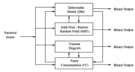
Figure 3.33. The hybrid segmentation engine.
We can derive a variety of hybrid segmentation methods by exchanging the filter used in each module. It should be noted that under the fuzzy connectedness and deformable models modules, there are several different filters that can be used as components. There are two methods of hybrid segmentation, derived from the hybrid segmentation engine: integration of fuzzy connectedness and Voronoi diagram classification (hybrid method 1), and integration of Gibbs prior and deformable models (hybrid method 2).
|
Politica de confidentialitate | Termeni si conditii de utilizare |

Vizualizari: 5403
Importanta: ![]()
Termeni si conditii de utilizare | Contact
© SCRIGROUP 2026 . All rights reserved