Studying the understory vegetation of Capitol Forest

Abstract

In conversations on the subject of modern forest practices, the phrase A tree farm is not a forest often comes up. While it is true that a working commercial forest has a shorter life-span than one that is excluded from human intervention, it is untrue that a commercial stand does not undergo to the same successional stages as a stand not subject to harvest. It has been a common forestry practice for many years to use understory indicator species to take a snapshot image of a stand during a survey and use that image as a rough descriptor of soil type, water availability, elevation, and a variety of other micro- and macro-climatic features that can be inferred from the presence or absence of a species in a stand. In this study, the goal was to establish a clear picture of successional stages in Capitol State Forest by comparing the understory composition in an ordered selection of even-aged stands from recently-planted clearcuts to mature stands that were marked for harvest. While the common understory species were dominant or even cosmopolitan throughout the study area, several of the species showed a strong trend to be present primarily in forest stands of certain ages. This suggests that understory analysis could prove useful in estimating stand ages without the necessity for potentially vectoring disease to individual trees through the use of increment borers.

Introduction

The study of succession in forest communities has been a subject of debate for many years (Clements, 1936 and Gleason, 1926). However, it is generally understood that as a forest stand develops from a primary-successional stage to a mature stand, it undergoes a series of compositional changes, both in the understory and in the overstory. Most of the literature available on the subject focuses on the overstory, as that is where the commercially-important species are located. Literature referring to understory species typically focuses on broad plant associations and, based on these associations, the inferences that can be made about soil, water, and other biotic and abiotic factors that influence the stand. Traditional forestry practice uses increment borers to drill into the tree and retrieve a core sample that can be used to count the annular rings, thus measuring the age of the tree. This is invasive and represents a possible vector for disease in trees drilled using the aforementioned method. In this study, conducted in Capitol State Forest, an idea was explored which suggested that understory species representing specific successional stages might be used to determine the age of a stand non-invasively.

Capitol State Forest is located in the Southern area of the Puget Sound, Washington, and is a popular destination for outdoor enthusiasts. Geographically, the forest is located within the Black Hills and includes Larch Mountain, Fuzzy Top Peak, Rock Candy Peak, and Capitol Peak. Capitol Forest is managed by the Department of Natural Resources and is the largest forested property they manage, covering 91,650 acres across Thurston and Grays Harbor Counties. Two small areas within Capitol Forest are privately-owned. 120 acres are broken into single family residences while Weyerhaeuser owns 120 acres on Larch Mountain. Capitol Forests boundaries include Highway 8 on the North side, the Black River on the East side, and Highway 12 on the South and West sides (Department of Natural Resources et al. 2005).

Tree species such as Douglas-fir, Western hemlock, Red Cedar, and Red Alder, as well as a lush understory, compose the most frequently-encountered plant communities of Capital Forest. Within Capitol Forest, elevations vary widely, the Chehalis River lowlands representing the bottom end of the scale at 200 feet and the top of Larch Mountain representing the opposite end of the scale at 2,660 feet. This diversity of terrain offers a broad variety of recreational opportunities. Public recreation sites are primarily situated near major rivers or streams. Clay-based soils in the area retain water, causing muddy conditions during wet months. As a result, only hiking and mountain biking are allowed during the winter season to preserve fragile soils on forest trails (Department of Natural Resources et al. 2005).

Todays Capitol State Forest is made up forest stands of different ages due to clear-cutting over the decades. Logging in the area began in the late 1840s. Before that time, the area was covered in old-growth trees with diameters of 8 to 12 feet and heights varying from 150 to 250 feet. Though the earliest settlers in the area took up land claims on prairie land, later settlers soon found that much of the best farmland was covered by these enormous trees. When these trees were felled, they were cut into shorter log lengths and moved into piles. These piles were then set on fire, after which the land around the stumps was tilled and called free land (Felt 1975). This was the beginning of clear-cutting in the Capitol Forest area. Soon after, loggers and timber companies made their way into the region, a pivotal event in Pacific Northwest history.

By the 1920s public concern over perceived forest exploitation arose, directed at lumbermen in the Pacific Northwest. The common opinion was that the timber companies policy of cut out and get out was beginning to harm the landscape. Foresters and conservationists with a more farsighted view of lumber practices were becoming better-known and better-respected by the public. Comparisons were made between then-contemporary West-coast forestry practices and East-coast forestry practices where entire forests of pine had been wiped out (Felt 1975).

Though logging practices of that time have been greatly criticized, the logging community itself cannot accept all the blame for those practices. While it is true that the timber companies could have planted new trees after logging a mature forest, the desire to clear land for farming brought visions and efforts predicated on millions of acres of stumpage being converted into livable family farms. At the time, this seemed much more economical than planting and growing trees (Felt 1975).

Eventually, in 1933, then-president Franklin D. Roosevelt made reforestation a household word in his famous fireside chats to the nation. Roosevelt was instrumental in the creation of the Civilian Conservation Corps, composed of young men from economically distressed cities and towns, who worked on various public projects. One of their more important projects involved working in the woods building trails, bridges, roads, fire-lookout towers, and parks. They also fought fires, cut snags, and planted trees. The Civilian Conservation Corps was the first government-backed program to get the public involved in rehabilitation and reforestation of timberlands (Felt 1975). It was largely through the efforts of the Civilian Conservation Corps that Capitol Forest became an actively-managed stand.

Since Capitol Forest is a working forest where trees are harvested while also providing recreational use, it has been officially named a multiple-use area under the jurisdiction of the Washington State Department of Natural Resources. Resource management and public use have proven to be compatible. Funds from Land Water Conservation Fund and Department of Natural Resource funds made it possible to create many areas dedicated to public recreational use (Felt 1975).

Because of the history of the area, there is much opportunity for studying regeneration of vegetation in Capitol Forest. This study began with the observation that following a clear-cut in Capitol State Forest, the understory composition changes as the stand ages. That is to say, following a disturbance, the understory develops through several successional stages before the stand is harvested again. Further observation suggested that there may be a way to compare stand age to understory composition and be able to make an educated guess about the age of a stand not from the size of the trees in the stand but rather from the smaller plants present on the ground. In each stand, both common and scarce understory species were tallied by percent coverage. This led to some interesting conclusions.

Methods

In studying the understory vegetation of Capitol Forest, it is to be understood that this is not a pristine, primeval forest; rather, this is a working forest that is subject to regular clearcuts. Assuming a 50-year growth cycle between clearcuts, stands for this study were chosen along main roads based on a best-guess estimate of their ages. Given this assumption, Early successional stages are defined as 5-15 years after a clearcut, Middle successional stages as 16-35 years, and Late successional stages as 36-50 years after a clearcut. This is the nomenclature that will be used throughout this paper.

Each stand chosen for the survey was marked by the roadside with a uniquely-patterned flagging tape. The age classes used for this study were 0 years to 50 years at five-year intervals. In each stand two plots with an area of 0.004 ha were surveyed and marked with an orange pinflag to define the plot center and to facilitate reproducibility. Plots within stands were chosen based on a few simple criteria:

The plot cannot be close enough to a road or the edge of another stand that it will be affected by the edge of these other features.

The plot should be more-or less representative of the whole stand; that is, a plot should not be selected due to unique or cool features that would falsely represent the stand as a whole.

The two plots within a stand should be separated by a distance great enough that the data from the two plots together accurately represent the stand as a whole.

Recent disturbance such as commercial thinning is cause for rejection of a stand. Pre-commercial thinning may or may not be cause for rejecting the stand as a whole, depending on the degree to which a stand has been modified by the thin. For example, one stand was rejected because all Red Alder (Alnus rubra) within the stand had been selectively removed during the previous season. At least one other stand was kept because the debris from the pre-commercial thin was many years old and represented very little downed woody debris to shade or otherwise alter understory composition.

Each plot within each stand was subjected to a rigorous survey, consisting of a series of standardized steps. Plot selection, in accordance with the above criteria, was the first step. The plot pole was driven into the ground to establish plot center (See Fig. 1), and a pinflag placed alongside the plot pole to mark the location (See Fig. 2). The second task upon establishing each plot was to note the aspect and slope relative to plot center, and from the same point, the azimuth and distance to the flag marking the stand on the road. The next step was tallying all nearby overstory species by percent coverage with a mind toward the area that a trees shadow would be likely to affect the light hitting the ground within the plot at midday. This was also done by best-guess, as the overstory was not the primary concern in this study, and was used primarily to differentiate between stands dominated by Douglas-Fir (Pseudotsuga menziesii) and stands dominated by Western Hemlock (Tsuga Heterophylla). Some thought was given to the idea of canopy closure but for the purposes of this study it was determined that the aforementioned best-guess estimate was sufficiently accurate for describing the effects the overstory shade would have on the understory composition.

The plot poles themselves were constructed of standard tool handles with cement nails hammered into their shaft and the heads cut off. Both of these materials are available at any hardware supply store. The cement nails allow the pole to be jabbed into the ground far enough that they will withstand the pull from the string representing the radius of a circle covering an area of .004 ha. It was determined through experimentation that it was necessary to cut the head off of the nails in order to allow the pole to be easily driven into soils of varying compositions without encountering either undue resistance to initial penetration or undue resistance to removal of the pole upon completion of data collection. These poles proved themselves highly effective for their intended purpose.

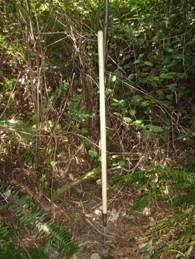
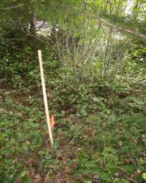
Figs.1 and 2: Plot pole and Pinflag marking plot pole

A string was constructed with a loop at both ends, one to go around the plot pole and one to go around the users wrist, with a knot marking 11.8 feet, which is the radius of a circle with an area of 0.004 ha. 11.8 feet was measured using the feet decimal scale on a standard Spencer Loggers Tape. Several types of string were tried before settling on cotton cord and polypropylene twine, depending on user preference. There was some trouble early on with the strings tangling badly. Several varieties of nylon twine were rejected for this reason. The string, pulled taut, was used to swing an arc of the prescribed distance, allowing close inspection of both common and scarce species on the plot in a rapid and reproducible manner. Steep slopes were corrected for by holding the string high or low on the pole as necessary to keep the string level. (See Fig. 3)

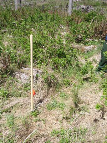
Fig. 3: Plot Pole, Pinflag, and String Extended

All species data were collected in this manner.

The following is a map of stand and plot locations. This and all associated maps were created in ArcMap 9.1. All of these map layers were collected from freely-available data on public servers on the internet owned by various government agencies. It is composed of a DEM raster image, road and water layers, and several manipulations of those primary layers. (See Fig. 4)

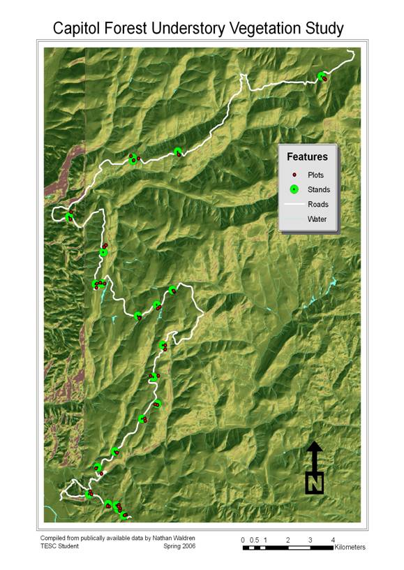
Fig. 4: Stand and Plot Locations and Route

In the field, these data were collected for each plot: Stand age and number, plot number, slope and aspect at plot center, azimuth and distance to the flag on the road marking the stand, major overstory species and coverage, major understory species and coverage, and a list of minor understory species found within the plot radius. In the field the minor species were listed as <5% coverage by area.

For simplicitys sake, species names were listed using the Codon convention, in which the first two letters of the genus and the first two letters of the specific epithet, forming a four-letter abbreviation unique to a species. In the event that two species share the same pairs of letters, they are numbered. A key to codons is included with this paper.

Once entered into Excel for data analysis it was discovered that the less-than symbol (<) is not a recognized operator, so those values were changed to 1. This changed the values for minor understory species to an essentially binary value: 0 represented the absence of a species on a plot, and 1 represented the presence of the same.

Major understory species that had coverage of greater than 5% by area were analyzed graphically using a Cartesian plot and an overlaid trendline representing a regression. Three regressions were used for each species: linear, second-order polynomial, and sixth-order polynomial. In all cases the latter provided the finest resolution but not necessarily the most useful data.

Minor understory species were graphed by frequency of occurrence rather than by percent coverage. A moving sum of the six cells closest to each cell was used to group events of a species occurrence into bunches; these bunches then approximated the likelihood of encountering that species on a stand of a given age. This method was required to make a graph out of these essentially binary values. Otherwise, graphing by coverage, the graph would have shown a straight line across the value of 1.

Future analysis of these data should include a comparison of slope, slope location, and aspect to these frequencies of occurrence.

Results

The data that resulted from this study came in primarily two forms: percent coverage vs. age, and frequency of occurrence versus age. In the species which were sufficiently abundant to be graphed by percent coverage, both graphs will be displayed. For the species which were sparse enough to only be visible as an occurrence event, only the frequency graph will be shown.

Sword Fern (Polystichum Munitum): nearly cosmopolitan throughout the study area, this species shows a peculiar trend from the earliest age class to the latest. By % coverage, the trend, graphed as a linear regression, is to increase slightly over time, while by frequency of occurrence, the trend is to decrease over time. (See figs. 5 and 6)

Fig 5: POMU Coverage vs. Stand Age (linear regression)

Fig 6: POMU Frequency of Occurrence vs. Stand Age (linear regression)

The graph of coverage % using the second-order polynomial regression shows a dip in middle-aged stands. (See fig. 7)

Fig 7: POMU Coverage vs. Stand Age (2nd order polynomial regression)

Dwarf Oregon-Grape (Berberis Nervosa) showed a similar pair of trends: increasing coverage vs. time contrasted with decreasing frequency of occurrence vs. time: (See figs. 8 and 9)

Fig 8: BENE Coverage vs. Stand Age (linear regression)

Fig 9: BENE Frequency vs. Stand Age (linear regression)

However, Berberis nervosa showed a rather interesting trend when percent coverage was compared to age using the sixth-order polynomial (See fig. 10)

Fig 10: BENE Coverage vs. Stand Age (6^th order polynomial regression)

The shape of this graph suggests that the plants present in younger stands were remnants of the understory that existed before the clearcut, and that they died off soon afterward, only to return as later successional stages developed.

At least one other species showed this same trend, that of residual populations immediately following a clearcut, which die off only to return later in the forests life.

Wood-Sorrel (Oxalis oreganis) (See figs 11 and 12):

Fig 11: OXOR Coverage vs. Stand Age (6^th order polynomial regression)

Fig 12: OXOR Frequency of Occurrence vs. Stand Age (6^th order polynomial regression)

By and large, most other species abundant enough to display as percent coverage graphs behaved very much the same as frequency of occurrence graphs. Here are two examples.

Red Huckleberry (Vaccinium parvifolium) (See figs. 13 and 14):

Fig 13: VAPA Coverage vs. Stand Age (linear regression)

Fig 14: VAPA Frequency of Occurrence vs. Stand Age (linear regression)

Salmonberry (Rubus spectabilis) (See figs. 15 and 16):

Fig 15: VAPA Coverage vs. Stand Age (linear regression)

Fig 16: VAPA Frequency of Occurrence vs. Stand Age (linear regression)

Some of the most interesting results came from the infrequent-to-rare species. For example, Ocean-Spray (Holodiscus discolor), Vanilla-Leaf (Achlys triphyllum), and Fir Clubmoss (Lycopodium selago) were all found in 50-year stands and nowhere else.

Less dramatic but more graphic results often took the form of species present early in stand life but absent late in stand life. The inverse is also true. Further, there were species that occurred frequently in middle-aged stands but at neither the beginning nor the end of stand life. This suggests a clear path through successional stages.

Here are two examples of species which occur early in stand life but are absent later.

Fireweed (Epilobum angustfolium) (See fig. 17)

Fig 17: EPAN Frequency of Occurrence vs. Stand Age (6^th order polynomial regression)

Foxglove (Digitalis purpureum) (See fig. 18)

Fig 18: DIPU Frequency of Occurrence vs. Stand Age (6^th order polynomial regression)

Here are two examples of species present in the middle of stand life but are uncommon at either the beginning or the end.

Star-Flowered False Solomons Seal (Smilacina stellata) (See fig. 19)

Fig 19: SMST Frequency of Occurrence vs. Stand Age (6th order polynomial regression)

Maidenhair Fern (Adiantum pedatum) (see fig. 20)

Fig. 20: ADPE Frequency of Occurrence vs. Stand Age (6^th order polynomial regression)

Finally, there were several examples of plants that were infrequent or absent in the early and middle successional stages of the stand but were frequently observed later in stand life. These are perhaps the best examples of succession illustrated by this study.

Here are two of those later-successional species.

Oak Fern (Gymnocarpium dryopteris) (See fig. 21)

Fig 21: GYDR Frequency of Occurrence vs. Stand Age (6^th order polynomial regression)

False Solomons Seal (Smilacina racemosa) (See fig. 22)

Fig 22: SMRA Frequency of Occurrence vs. Stand Age (6^th order polynomial regression)

There were a few species that showed odd behavior, such as multiple peaks in frequency, as seen through the lens of a sixth-order polynomial regression.

Red Huckleberry (Vaccinium parvifolium) (See fig. 23)

Fig 23: VAPA Frequency of occurrence vs. Stand Age (6^th order polynomial regression)

Vine-Maple (Acer circinatum) (See fig. 24)

Fig 24: ACCI Frequency of Occurrence vs. Stand Age (6^th order polynomial regression)

Discussion

Through the course of this study, it became quite evident that certain understory species displayed a marked preference for specific ages of stands. This supported the thesis concept that a correlation could be made between understory composition and stand age.

However, there were a few oddities and a few interesting sites that didnt really fit the cut-and-dried idea that X species understory composition equals Y age. One of these oddities was that in 40-50 year old stands composed purely of Western Hemlock (Tsuga heterophylla) the understory was often sparse or altogether absent. This is due to the highly competitive succession in young Hemlock stands; by the time the stand is 40 years old, it has self-thinned to a relatively small number of stems per acre, the canopy has closed, blocking light from reaching the ground, and most of the nutrients in the soil have been depleted. This understory absence can be quite conspicuous. In one such stand, there was an observable line between the sterile Hemlock understory and an unusual Oxalis/Corydalis association not observed elsewhere, and not listed in the applicable USFS Plant Association Guide. (See figs. 25-27)

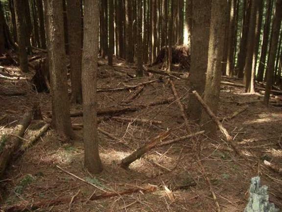
Fig. 25: Sterile Understory in Middle-Aged Western Hemlock Stand

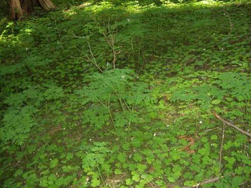
Fig. 26: Oxalis/Corydalis Association in Western Hemlock Stand

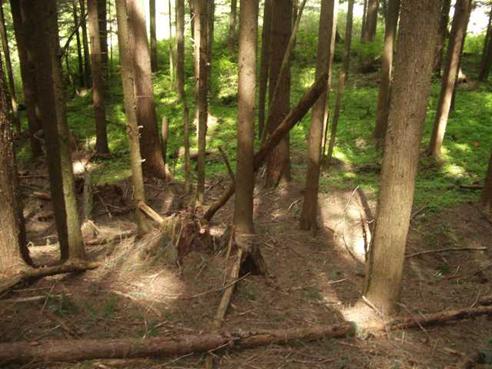
Fig. 27: Boundary between Sterile Understory and Oxalis/Corydalis association in Middle-Aged Western Hemlock Stand

Closer observation of this boundary suggested the possibility that water availability and drainage made this association possible. Close observation of this stand using a TIN (Triangular Irregular Network) projection of this stand showed that there was indeed an inflection point in the topography of the stand exactly where the line between the sterile understory uphill and the Oxalis/Corydalis association below it. (See fig. 28)

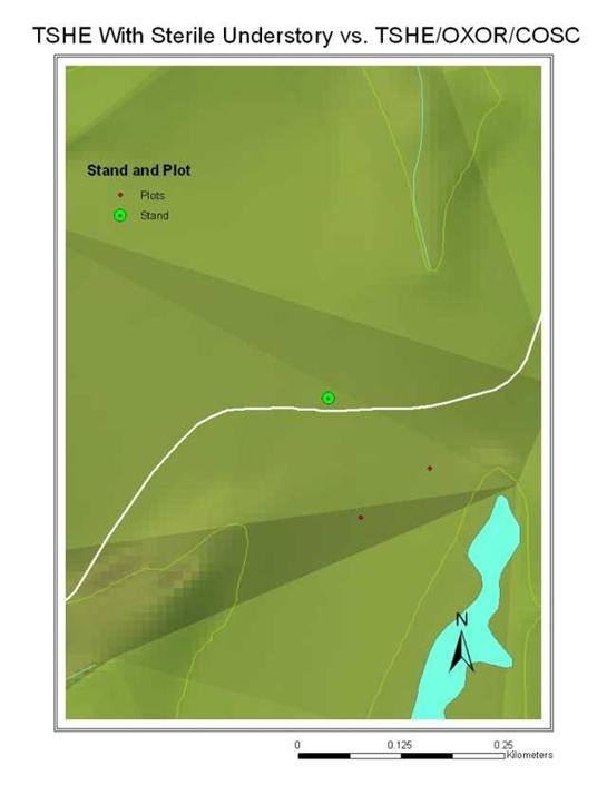
Fig. 28: TIN Projection of Western Hemlock Stand Showing Topographical Details

Another event that factored into the dynamics of many stands of many ages was occasional incidence of secondary disturbance. The experimental design of this study considered a clearcut to be a clock-resetting disturbance event, and, as such, overlooked several natural and unnatural events that commonly occur within a forest stand during its lifetime. Natural disturbance events which were evident within the study area included fire, lightning, windthrow, disease, and herbivory. Unnatural events were primarily limited to thinning, either commercial or precommercial. These secondary disturbance events often affect both under- and overstory. All efforts were made to choose stands that were not unusually affected by either the absence or presence of secondary disturbance events, but rather to choose stands that were representative of their age class within the area being studied. It should be noted that a different study area may well have required different selection criteria.

The disease most frequently encountered was Laminated Root Rot (Phellinus weirii), evident most commonly in the root balls of wind-thrown trees. In one stand the infection was widespread enough to have killed all the trees within a 30-meter radius. (See fig. 29)

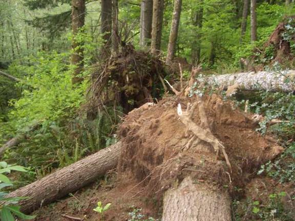
Fig 29: Trees Wind-Thrown due to Phellinus Infection

The characteristic features identifying Phellinus in the field are the separation of annular rings in broken-off roots, as well as the presence of a unique reddish-brown structure called Setal Hyphae. These features were present in nearly all wind-thrown trees found in the areas studied. In all cases, conspicuous conks were absent, differentiating this infection from Annosus Root Disease (Heterobasidion annosum) (See figs. 30 and 31)

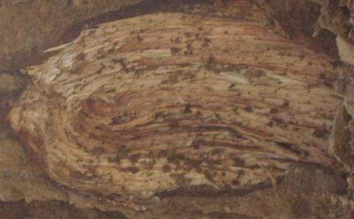
Fig. 30: Annular Ring Separation in Roots of Wind-Thrown Tree

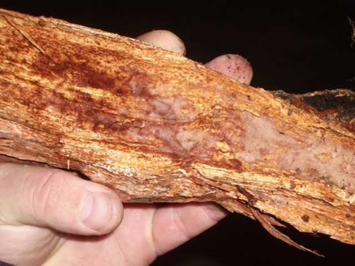
Fig 31: Laminated Root Rot Showing Detail of Setal Hyphae

Another occasional pathogen throughout this study area was Arceuthobium Dwarf-Mistletoe, evident by its characteristic Witches Broom structure on infected branches. As Arceuthobium is dioecious, each infection is the result of two other infections, one male and one female. (See figs 32 and 33)

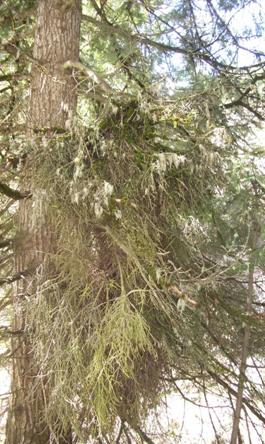
Figs. 32 and 33: Arceuthobium Dwarf-Mistletoe infections on Western Hemlock (Tsuga Heterophylla) and Grand Fir (Abies grandis)

Several stands showed evidence of low-intensity fire in the form of cat-face scars at the base of tree boles. This is differentiated from slash-burning in that the damage occurred within areas of standing timber. Much of the available literature on the subject of forest succession in the Pacific Northwest focuses on the effects of slash-burning on early- and middle-successional stands. Unfortunately, that data was unavailable for the purposes of this study and therefore cannot be used for comparison. (See fig. 34)

Fig. 32: Cat-Face Scar from Low-Intensity Fire In Standing Timber

Nonetheless, through analysis of raw field data it became evident that there is indeed a successional hierarchy, and that that hierarchy could be used to determine the age of a stand non-invasively. Some species are more useful as indicators than others. For example, Sword Fern (Polystichum munitum), which was nearly ubiquitous throughout the study area, showed little enough variation in either frequency or coverage to be apparent to the naked eye. Thus, it could not be used as an indicator of stand age. Several other species were clearly indicative of a general stand age (i.e. early, middle, or late successional) and could be used to predict the age of a stand. These indicators were more dramatic at the beginning and end of the sample age period, though there were many species that also showed both higher frequency and wider coverage in the middle of the sample age period. It is interesting to note that many of the species that showed the lowest percent coverage also showed the highest relative frequency by age. A few only occurred in early- or late-successional stands. These were the most useful indicators of stand age.

That said, these data are primarily useful in that they show snapshot images of stand composition across clearly-defined age classes and can therefore be expected to model with some accuracy the understory species compositions of other stands of the same age, within the same region. It is likely that a larger study would bear this out.

Conclusion

The methods used in this study are simple, yet robust. A single surveyor familiar with the flora of a given region could easily collect these same data in a different location and come to similar conclusions. That said, this method could be a useful tool in non-destructively testing the age of unknown stands without the need for the use of an increment borer to determine the age of individual trees, and by association, entire stands.

This would require a matrix of some sort where there is a criterion-matching scheme to determine a stands age to within an acceptable margin of error. This matrix would have to be composed of both minor and major understory species, and, like the USFS Plant Association Guides, would have to be tailored for a specific region. Fortunately, in the Pacific Northwest, at least, the regions are relatively easy to define geographically and relatively homogenous throughout each region. This could be used in the field either on paper or on a portable computer of some sort to simply describe the vegetation and physical conditions of a plot and to generate an age profile for the entire stand that is accurate within +/- whatever the tolerance of the algorithm allows.

This model would only work for even-aged stands. Burned-over or partially-logged stands with remnant trees remaining from prior stands would skew the data beyond the accuracy of any algorithm foreseeable within the limitations of this model. For this reason it is perhaps best to recommend using this method only in actively-managed stands.

To further test the validity of this model, a study of a larger sample size and geographic magnitude would be useful. This would also serve to decrease the significance of unusual stands and uncommon or rare species that might seem unusually common in a study of this size.

Future study should treat small geographic regions with this same method, as each microecology is different, even within a single stand. Broader geographic differences compound this problem, making it difficult to produce data that is applicable over any kind of distance.

Ultimately, the goal of this sort of study is to produce a sort of Site Index that can be used to definitively determine the age of a stand. This differs from traditional forestry methods in that rather than making assumptions about he whole stand based on the behavior of selected trees, these assumptions would be made from the whole stand. This would be a useful tool for foresters, floristic researchers, ecologists, and many other professionals.

One difficulty with this method is that it requires a good deal of training to be able to positively identify all species on a given piece of ground. Anyone attempting this sort of study should be prepared to spend a good deal of time in the pertinent local Flora identifying the oddballs that will inevitably show up from time to time. This is key, as these oddballs are often valuable indicators both of stand age and of soil, water, and nutritional conditions within the stand.

Literature Cited

Barbour, Michael G., Burk, Jack H., Pitts, Wanna D., Gilliam, Frank S., and Schwartz, Mark W. Terrestrial Plant Ecology. 1999. Menlo Park, Ca: Addison Wesley Longman, Inc.

Chang, Kang-tsung. Introduction to Geographic Information Systems. 2006. New York: McGraw-Hill

Clements, Frederic E. 1936. Nature and Structure of the Climax. Journal of Ecology 24: 252-284.

Creso, Irene. 1984. Vascular Plants of the Pacific Northwest. Tacoma, WA: Johnson Cox Printers.

Dyrness, C. T. 1973. Early Stages of Plant Succession Following and Burning in the Western Cascades of Oregon. Ecology 54: (1) 57-69

Felt, M. A. 1975. Capitol Forest: The Forest That Came Back. Washington State Department of Natural Resources. Pg. 1-75

Frelich, Lee E. Forest Dynamics and Disturbance Regimes. 2002. Cambridge, UK: Cambridge University Press

Gleason, H.A. 1926. The Individualistic Concept of the Plant Association. Bulletin of the Torrey Club 53: 7-26

Halpern, C. B. 1988. Early Successional Pathways and the Resistance and Resilience of Forest Communities. Ecology 69: (6) 1703-1715

Halpern, C. B., and Spies, T. A. 1995. Plant Species Diversity in Natural and Managed Forests of the Pacific Northwest. Ecological Applications 5: (4) 913-934

Hemstrom, Miles A., and Logan, Shiela E. Plant association and management guide Siuslaw National Forest. 1986. USDA Forest Service Pacific Northwest Region R6 Ecol Technical Paper 226-1986A

Henderson, Jan A., Peter, David H, Lesher, Robin D, and Shaw, David C. Forested Plant Associations of the Olympic National Forest. 1989. USDA Forest Service Pacific Northwest Region R6 Ecol Technical Paper 001-88

Hitchcock, C. Leo, and Cronquist, Arthur. 1994. Flora of the Pacific Northwest. Seattle, WA and London, England: University of Washington Press.

Holt, Vesta. Keys for Identification of Wild Flowers, Ferns, Trees, Shrubs, and Woody Vines of Northern California. 1962. Palo Alto, CA: National Press Books

Lide, David R. CRC Handbook of Chemistry and Physics. 1993: Boca Raton, FL: CRC Press.

Scharpf, Robert. Diseases of Pacific Coast Conifers. 1993. Washington, DC: USDA, Forest Service Handbook 521

Stoddard, Charles H. Essentials of Forestry Practice. 1968. New York: The Ronald Press Co.

Washington State Department of Natural Resources. Capitol State Forest Recreational and Public Access Plan: Background. 2005. DNR Technical Paper pg. 11-25

Capitol Forest Understory Vegetation Survey

Justin Kidulson and Nathan Waldren

Spring Quarter 2006

Appendix: Codon Key