Introducing the MIDAS Method of Technical
Analysis
In this, the first of a series of columns, we will introduce to the
community of technical analysts a new approach to charting the price history of
a stock or commodity. I call this technique the MIDAS method, an acronym for
Market Interpretation/Data Analysis System. It is designed to focus attention
on the dynamic interplay of support/resistance and accumulation/distribution
which are the ultimate determinants of price behavior. Indeed, a Midas chart
makes immediately visually apparent an unexpected degree of orderliness in what
might otherwise seem to be a random or chaotic process.
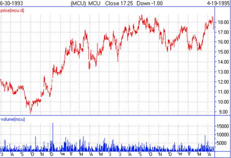
Take a look at the first of the figures. Here we have a standard price
and volume bar chart for Magma Copper as of the April 19, 1995 close. I do not
believe any of the familiar charting methods would contribute anything of value
to the interpretation of this chart. There are no clearly evident trend
channels, trendlines, support or resistance lines, etc. Indeed, after the
initial runup from 9 to 17, the subsequent sideways pattern appears to be
random and trendless.
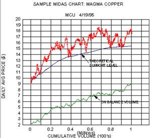
Now look at the Midas chart for the same stock. First observe that to
simplify things we only plot the daily average price (i.e. the average of the
high and low). More signifcantly, we plot the prices vs. CUMULATIVE VOLUME
rather than time. This has the effect of giving less visual weight to periods
of relative inactivity (e.g. Feb 1995) since the lower cumulative volume
increase during such a period compresses the daily points into a smaller space.
(We will see later on why it is important to deemphasize periods when there is
little alteration of the ownership profile of the people holding the stock).
Next, observe the curve marked 'theoretical support level',
and in particular how this corresponds precisely to the trend reversal points.
You might think that in some sense the theoretical support curve has been
'fitted' to these reversal points, much in the same way that
trendlines are fitted to bar or point and figure charts. Remarkably, this is
not the case; the theoretical support curve is determined a priori, has no
adjustable parameters and follows from a very simple equation. In a later
column I will derive this equation from a quantitative consideration of a few
universal features in the psychology of the trader. For now just take my word
for the fact that the theoretical support curve was constructed in a
universal fashion from the raw price and volume data.
From the standpoint of practical trading, the important thing is that
the price trend reversals (eight in all) all occurred precisely where they were
expected to. This by itself both confirms a primary bull trend, and provides
low risk entry points for long positions. One simply waits for the price to
approach the support curve and jumps on board at the first indication of a
'bounce'. (Where to sell is of course another matter which we will treat
at length in future columns).
But how strong a bounce are we to expect, or to put it another way, how
strong is the underlying bull trend? To assess this, we add one final feature
to the Midas chart, viz. a minor variant of Joe Granville's on- balance volume
('obv'). This curve is constructed by adding today's volume to the
(accumulated) on-balance volume if today's average price exceeds yesterday's
average price, subtracting it if it is less, and not changing the on-balance
volume if there has been no day to day change in average price. (The absolute
scale of the obv curve is immaterial and is simply adjusted to fit on the same
chart as the price). The value of obv is that it makes
immediately clear whether a stock is undergoing accumulation or
distribution.
In the present example we see that obv is in a definite upward trend
(accumulation) and that the obv trend continues even during periods of sideways
price action. This is ideal bullish confirmation of the price trend. To
summarize the ground we've covered in this first brief introduction, we have
shown how price and volume data for a specific stock can be displayed in a new
fashion which makes immediately apparent an underlying trend that is all but
hidden in a conventional chart of the same data. It is a totally remarkable
circumstance that this general approach to charting appears to be of practical
value in most markets for which I have been able to test it against price and
volume data. In my next column I'll give a few more examples of Midas charts
for stocks of current interest. When we have examined together several such examples
and have thereby developed a familiarity with this new way of looking at
things, there should be sufficient motivation to delve more deeply into the
mechanics of generating the theoretical support curve. In so
doing, we will come to discover other unexpected regularities in what
has often been dismissed as random walk
processes. Stay tuned!
In the first article of this series we introduced the Midas chart as a
new way of displaying historical price and volume data. Containing three
essenial elements: daily (average) price, a theoretical support level, and on
balance volume - all plotted vs. cumulative volume rather than time - the Midas
chart provides a hitherto unavailable framework for categorizing and in many
cases understanding the dynamics of price behavior.
Specifically, in this approach,
it is the price relative to the theoretical support curve that determines the degree
to which the stock or commodity is overbought or oversold. This is in contrast
to the more familiar methods of technical analysis which focus instead on price
relative to moving averages, linear trendlines and/or previous tops and
bottoms. The on balance volume in turn provides a measure of the
'strength' of the support curve, i.e. whether it will hold or be
penetrated.
In this and future articles, we will develop these concepts by studying
specific examples in detail. So let's
turn first to the Midas chart for Stone Container below. Note first how well
the theoretical 'primary' support level curve predicted the actual
trend reversal points. (Traditional technical analysis would have anticipated
that the pullback from the peak at around 21 would be stopped at about 17 - the
previous peak).
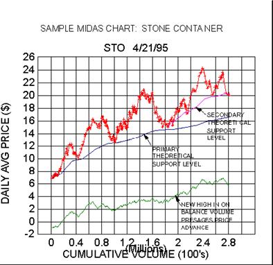
Next note how the movement of the on balance volume to new high ground
correlates with the
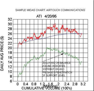
subsequent move to new highs in the price. This is in contrast to the
second example below, Airtouch
Communications, where the marked declining trend of obv correlates with
the subsequent penetration of the
theoretical support level. In the absence of the obv data, one might
have expected the support level to 'hold' and
give rise to a new upward price leg since up to that point it had indeed
provided support just as in Stone
Container.
Returning to Stone Container, note finally that we have introduced a new
feature of the Midas method:
the concept of a hierarchy of support levels. We thus speak in terms of
a 'primary' support and a
'secondary' support. (While we have yet to present the
equations for these theoretical curves, for now we can
say that both the primary and secondary support curves are generated by
the same algorithm.) Indeed, in
articles to follow we will show examples of strongly trending stocks for
which one can clearly distinguish primary,
secondary, tertiary and even fourth order support levels.
To introduce some Midasspeak, a Midas theorist would describe Stone Container
thusly: 'STO is in a
primary bull move, with a thrice validated primary support level. It has
currently pulled back to and is
pausing at a doubly validated secondary support. No deterioration in the
upward trend of obv is yet evident, so
the expectation is that the secondary will hold and the price will
resume its upward motion. If the secondary fails
to hold, the price would be expected to decline at least to the primary
support level at about 17.'
Even though we have only looked at three Midas charts in this and the
previous article, there should
already be a change in the way we look at a conventional price vs time
bar chart. One should focus on the
trend reversal points and see whether one can visualize a series of
support curves to which they might
correspond. To facilitate this visualization, in the article to follow
we will transform Midas charts from the
cumulative volume to the time domain. In addition, since these three
examples are all in contemporary real time,
we will revisit them later to see how useful the Midas framework has
been in characterizing their subsequent
behavior.
In the previous article in this series, we introduced the concept of a
hierarchy of support levels,
according to which trend reversal points can be identified with finding
support at one member of a
group of theoretical support curves (labelled 'primary',
'secondary', 'tertiary' etc. according to
seniority). This is illustrated in the Midas chart for Royal Carribean
Lines (RCL), where we have plotted three
such support curves. We have also called attention in this chart to
another example of the utility of including the
obv as a leading or coincident indicator of price trend change.
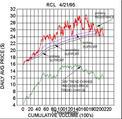
Note also that for the first time we have shown a theoretical RESISTANCE
curve. In point of fact, there is
complete symmetry in the Midas method between support and resistance!
The theoretical resistance curve is
generated by exactly the same algorithm as the support curve(s).
As a general rule, when one observes multiple confirmations of a
relatively 'young' resistance curve,
together with a change in the trend of the obv - as in the RCL example -
then the expectation is that the
hierarchy of support levels will be violated one by one and replaced by
a new hierarchy of resistance
levels defining the new primary bear trend. This is on the verge of
happening in RCL which is at a crossroads
as of 4/21/95.
Note RCL has stopped at the primary support level and that obv has not
yet broken down into a new
low (in fact it is slightly higher than it was at the previous contact
with the primary). RCL could bounce
from here and again challenge the primary resistance. In fact we often
encounter cases where the price is
'squeezed' between primary support and resistance curves, a
silent mortal combat that is usually not evident in
the conventional charts. If the price does convincingly penetrate the
primary support, on the other hand, with
corresponding new low in the obv, then the probability is high that the
primary bull move which carried RCL from
16 to 30 is over.
A second example of the completely symmetrical roles played by the
theoretical support and resistance
hierarchies in the dynamics of a major trend reversal is shown in the
Midas chart for Digital Equipment
(DEC). The near-coincident penetration of the primary resistance, the
breakout into new high ground of the obv
and the first validation of the young secondary support (at a cumulative
volume of about 2.65) all confirmed the
expectation that a primary bull trend was underway. Conventional
technical analysis, on the other hand, might
have interpreted this as merely a 'normal' 50% retracement of
the drop from 43 to 19!
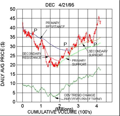
Now note the areas marked 'P' in the DEC chart. P stands for
'porosity' which is the term I use to
characterize situations when a 'bounce' from a support or
resistance level is not 'clean' in the sense
that some relatively small penetration occurs before the expected trend
reversal. Perhaps 'elasticity'
would be a better term than porosity, since the S/R (an abbreviation for
'support or resistance' which we shall
henceforth use) level can be imagined to have some 'give'
rather than being rigid. Or one could just say that the
Midas method is after all a simple approximation to a more complex and
less deterministic reality.
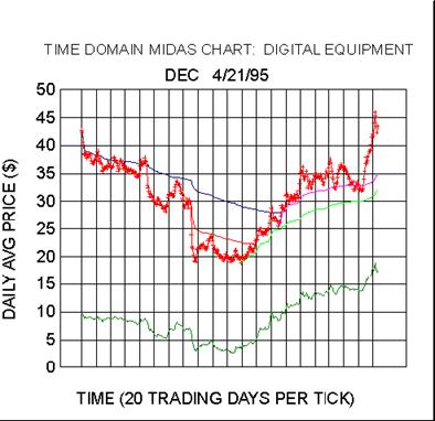
Finally, to deliver on a promise made at the conclusion of the preceding
article, in the next graph we
show what the DEC Midas chart would look like if we plotted everything
versus time rather than
cumulative volume. In this mode of representation, the S/R levels are
seen to be 'jerky' and therefore are
difficult to visually extrapolate, whereas in the cumulative volume
domain they are relatively smooth and
continuous. Thus we prefer to work with cumulative volume instead of
time, although this is not always possible.
When we wish, for example, to introduce the Midas theoretical S/R levels
into commercial charting software
packages - which we will in fact do in a later article - we are stuck in
the time domain since such packages have
no flexibility in choice of abscissa. Our hope of course that these
articles will create sufficient interest in the
Midas approach to motivate the software authors to generate Midas
upgrades to such packages!
It is worthwhile to pause for a moment at this stage of the development
to delineate what it is we are
trying to accomplish with the Midas method of technical analysis. Our
objective is best explained by
analogy to the understanding of atomic spectra as it existed in the 19th
century, before quantum mechanics.
Spectral lines had been observed to group into families according to
their wavelengths, and numerological
relationships such as the Balmer series were empirically fitted to the
observations. Some order was thereby
imposed on the complex spectra, but without any understanding of the
underlying reason why these formulae
should apply. It wasn't until the spectral lines were identified with
transitions between discrete atomic energy
levels, that it became clear that an understanding of the spectra would
follow directly from an understanding of
these levels. The levels were the fundamental reality, and the spectra a
secondary consequence.
In like fashion, we view the hierarchy of S/R levels as being the
fundamental reality underlying stock
price behavior, and do not believe that a coherent model of this
behavior is possible without them. It is
therefore not surprising that extant computerized trading systems which
do not include this reality are generally
ineffective. Even with the powerful tools of neural networks and
adaptive systems, one is in effect finding the
optimum square peg for a round hole.
With our focus on the relationship between price and the S/R hierarchy,
we have a powerful taxonomic
tool to identify universal patterns of behavior exploitable for trading
profit - patterns that would not be
discernable from a consideration of the prices alone, i.e. without
reference to the S/R hierarchy.
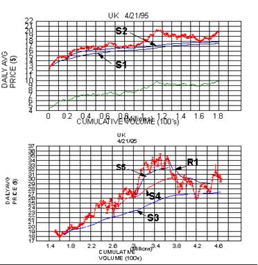
We can illustrate this by a detailed consideration of the anatomy of a
complete bull move in a stock. The
first figure shows the Midas chart for such a move in Union Carbide
(UK). The chart covers 638 trading days
ending on April 21, 1995, or about 2.5 years. Plotted on the chart are
four support levels S1..S4 (a numbering
shorthand we will henceforth use for simplicity).
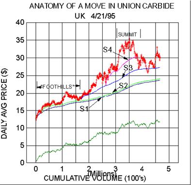
We turn first to the start of the move and have identified what I call
the 'foothill' pattern. Anyone who
has approached the Sierras in Calif.
from the west has noticed that one first traverses a series of gently rolling
hills whose rate of rise is quite gradual compared to those of the
mountains ahead. Clearly if one can identify a
stock move in the foothill stage, one can capture the bulk of the price
appreciation.
In the top half of the second figure we therefore put a magnifying glass
to the foothills, a period
covering about 230 trading days. Note how beautifully the prices ride
along the secondary support S2, and
how the obv is poised to break out into new high ground. Referring back
to the first figure we see this is just
prior to the start of the sharply climbing price 'mountain'.
THIS FOOTHILL PATTERN HAS PROVEN TO BE THE MOST USEFUL TOOL FOR SPOTTING
LOW
RISK/HIGH REWARD ENTRY POINTS FOR INTERMEDIATE TERM LONG POSITIONS. It
is noteworthy that
without reference to the support levels, very little seems to be going
on in the foothills. For months at a time the
price is confined to a very narrow range and it is only if one is
trained to look for a pattern of repeated bounces
from a theoretical support level that the situation can be recognized.
Imprint this graph firmly in your mind, for we
will see this behavior over and over again. Indeed, in future articles I
will call attention to such occurrences in
real time, as they are unfolding!
The lower half of the second graph focuses on the summit of the price
mountain. What I wish to
emphasize here is that in the final push to the summit, the applicable
support level was of FIFTH ORDER. As a
general rule, when one observes such high-order support levels holding
up prices, the end is known to be near.
One then pays particular attention to ancillary indications of topping
behavior, such as the head and shoulders
formation evident at the UK
summit, to time one's selling. (We will present other tools for identifying
selling points
in future articles).
Note how the drop off from the summit is bounded by the resistance level
R1 for several months until it
in turn is penetrated by the recent bounce from S3. What does the future
hold from this point on? Our best
guide is the obv curve of the first graph, where we see that obv is
still quite close to its high. This would tend to
indicate that there is still some life in the bull move yet, and that
another leg to new high prices may be in the
offing, perhaps after one more pullback to and bounce from S3 at about
27 1/2. Indeed, the penetration of R1
makes this the likely scenario. We'll revisit UK in a future article to see how
things work out.
In the previous article we emphasized that our primary goal with the
MIDAS method is to provide a
means of characterizing price behavior which is based on underlying
realities rather than ad hoc
empiricism or numerology. This is fundamentally a scientific question,
quite apart from the tactical matter of
utilizing such knowledge for trading advantage. In a broad sense we may
thus distinguish between what might be
called the scientific and the engineering aspects of MIDAS, where the
former encompasses the quantitave
'laws' which give rise to the S/R hierarchies, and the latter
refers to practical trading rules and techniques based
on this understanding.
We made a start on the engineering side by showing how the
'foothills' could be recognized and used
as a low risk/high reward entry point for intermediate term long
positions. Here the window of opportunity
is quite wide in time since the foothills have a typical time scale of
the order of months and it is merely a matter
of scrutinizing a sufficiently large number of stock charts to find some
likely candidates. Once one gets used to
spotting foothill behavior in the gentle undulations of conventional bar
charts, a few hours each month leafing
through a book of daily basis stock charts will suffice to identify at
least 30 or 40 such candidates justifying
further analysis using quantitative MIDAS methods.
The reversal of a long consolidation or bear leg within a primary bull
move, via a bounce from S1 or S2
provides an even better trading opportunity since the gains come much
more quickly and the price
objectives are well defined. (At a minimum one expects to reach the
nearest resistance level, usually an
R1 or R2. If this is penetrated then the next objective is the previous
high.) The window of opportunity is
however much shorter, typically a few days to a few weeks. Furthermore,
for any given stock there may only be
one or two such opportunities per year.
Thus while MIDAS methods could be used on single stocks to determine
good entry points for long
positions suggested on fundamental (as opposed to technical) grounds,
the trader will monitor many
stocks ( of the order of hundreds ) in order that sufficient
opportunities will be found to keep capital off
the sidelines. To facilitate the application of MIDAS to a large
universe of stocks in real time, we have
developed some interesting techniques for compressing a fairly complete
MIDAS characterization of a given
stock into a few ascii characters.
This is illustrated in the first figure which contains a Midas chart of
EMC Corp. By now this should be so
familiar that no commentary is required. (Although one cannot refrain
from marvelling at how well the trend
reversals are anticipated!). Above the chart is a single line of ascii
characters and its associated legend.
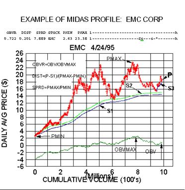
Note the line of dashes bounded by an 'l' (for low) and an
'h' (for high). This represents a price range
extending from 2.63 to 23.38 in this case. The capital 'S'
denotes the relative position within this interval of the
primary support level S1. The corresponding positions of the secondary
and tertiary supports are indicated by
lower case 's''s. The asterisk is the average price for that
particular day. Thus this so-called MIDAS Profile
shows the number of S/R levels (resistance levels use 'r'
instead of 's'), their relationship to each other and to
the latest price, as well as where they all stand in relation to the
high and low for the historical period in
question.
Two further features may be simply added to convey even more
information. If a given S/R level is
particularly well 'validated' (i.e. it has successfully
predicted several trend reversals with little porosity), we can
underline the symbol as we have done for S2 (or it could be made
boldface if the software and printer permit).
In addition, if the asterisk should happen to coincide with an S or an
s, we can replace it with a >> or a > (or <<
or <) respectively. This has the effect of immediately calling
attention to the fact that the price is at an S/R level
and perhaps ready to bounce.
In addition to this pseudo-graphical technique, we generate the three
ratios defined in the graph. OBVR
is an obv ratio measuring how far the obv has retreated from its peak
value. The closer OBVR is to unity, the
more bullish the outlook. DIST (standing for 'distension') is
a normalized measure of how close the latest price
is to S1. SPRD (for 'spread') measures the volatility of the
stock over the historical period of study.
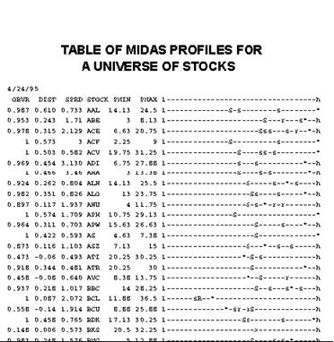
Trading rules can be developed based on these three quantities. For
example, one can only enter long
positions when OBVR exceeds a certain threshold, DIST is less than
another threshold (i.e. close to S1 and
ready to bounce) and SPRD is greater than a third threshold (to weed out
stocks that are not volatile enough to
have a sufficient potential reward). Now a neural network trained on
these inputs might have some hope of
success!
For a group of stocks, one would then generate each day a table such as
that shown in the second
figure. With a little practise one can thereby review a few hundred
stocks in a matter of minutes to identify
interesting opportunities.
Another visual technique is the scatter plot shown in the third figure.
Here, each stock is assigned an ascii
symbol which is then positioned in the plane according to its OBVR and
DIST coordinates. DIST is the horizontal
axis, where we have placed 'oversold' corresponding to DIST=0,
and 'overbought' when DIST=.5. (The reason
for the latter choice will emerge when we develop the equation for an
S/R level).
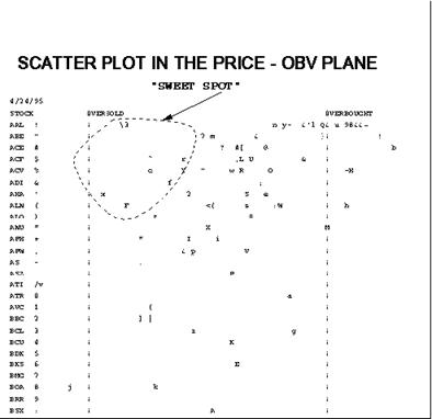
Since we wish to easily spot situations when a stock is close to S1 with
a high OBVR, we need merely
watch the region marked 'sweet spot' and then have a closer
look at the MIDAS charts for those stocks
which show up there.
On a more sophisticated level, one can program customized trading
systems based on MIDAS for
inclusion in one of the many commercial trading software packages to do
such scans automatically,
aided perhaps by additional filtering using other tools of conventional
technical analysis. I'll give some
examples of this in a later article.
Our goal in the articles to this point has been to establish the
credibility of the S/R hierarchy on the
basis of its manifest ability to bring a degree of order into the
apparently random zigzag patterns of
stock prices. One measure of the power of any scientific theory is the
degree to which many observations can
be accommodated by the fewest principles ('Occam's Razor'). In
the present context, this means fitting the set
of trend reversal points - the zigzags - with a small number of S/R
levels, all derived from a single simple
algorithm (which will be derived in the article immediately following
this one). For now we wish to exhibit a few
final important properties of the S/R levels, and to discuss some
limitations of the Midas method.
Turning first to the Midas chart for Tandem Computers (the obv curve was
omitted so we can observe
finer structural details of the price behavior) we have plotted a
primary, secondary and tertiary support
and two primary resistance levels. Note first that we discontinued the
first R1 as soon as it was convincingly
penetrated. S/R levels do frequently 'wear out' for reasons
which will be clear when we present the S/R
algorithm. A new primary resistance level is introduced to accommodate
the retreat from the second price peak.
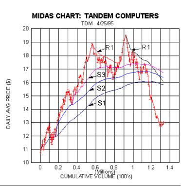
Next note that on the other hand, the support levels S2 and S3
maintained their viability (i.e. their ability
to fit subsequent zigzags) after having been penetrated. Generally
speaking, the older a level is, the more
this tends to be the case.
Another interesting feature which can be seen in the S3 curve is the
familiar property that a support
level which has been violated becomes a resistance level when apporached
from below. The reason for
this behavior will also be clear when we derive the S/R algorithm.
Most importantly please take note of and remember the catastrophic
failure of S1 to halt the price
decline to below 13. This underscores the fact that the future is after
all not cast in concrete. The perceived
prospects of stocks are subject to abrupt and unforeseen changes. While
an existing S/R hierarchy may be
strong enough to bound the price variations within a given set of
assumptions in the market regarding the
prospects of the company, its group and the market as a whole, any
sudden shift in this paradigm can call into a
play a totally new price dynamic.
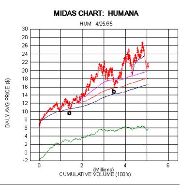
Fortunately, this is not always necessarily the case as may be seen in
the Midas chart for Humana. Note
first that as with Tandem, the level penetrations at points
'a' and 'b' did not invalidate their subsequent viability.
More significantly, note that the recent sharp decline (brought about by
a sudden reappraisal of all health care
providers, or what we may call a group paradigm shift) was halted - at
least for now - at a (mature and
well-validated) S3.
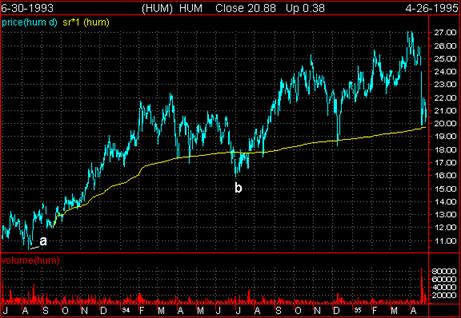
Finally, to come full circle, in the first article we showed a
conventional price and volume bar chart and
followed it with a Midas chart of the same stock (Magma Copper). So now
let's look at a bar chart for
Humana upon which we have superimposed the Midas S3 support level. The
results speak for themselves. The
clear fact that so many apparently unrelated points of trend reversal
can be understood with reference to a
single theoretical S/R curve testifies to the power of the Midas method.
Indeed, recalling the analogy in article
#4 with atomic spectra, it is perhaps not too much of a stretch to view
the Midas method as 'price
spectroscopy'!
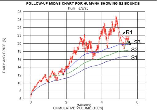
POSTSCRIPT:
Article 6 was written on 4/25/95. In view of the delay in its
publication, I thought it might be interesting to see
what happened to Humana in the subsequent days. The results are shown in
the fourth figure. Support was
found at the secondary level S2 (actual low for the day was 17 7/8;
recall that we plot the average price) and
the bounce carried up through the incipient resistance level R1. Humana
is now riding on a tertiary support level
S3.
In the preceding six articles, it has been shown that the support and
resistance levels associated with
points of trend reversal in the price of a stock can be classified with
respect to a hierarchy of
theoretical curves. It is now appropriate to derive the simple algorithm
giving rise to these curves from a
consideration of familiar aspects in the psychology of the market
participants. After all, it is precisely the
dynamic interaction between the greed and fears of those who already
hold the stock and those who wish to
become owners that determines the price at which supply and demand find
at least temporary equilibrium.
One can approach the problem from both the supply side and the demand
side with remarkably similar
results. First consider someone who already has a long position in a
given stock. What will motivate this person
(the 'owner') to sell? If the stock is held at a profit, the
more substantial this profit is the greater the temptation
to take it. If - not having taken such profit - the owner sees the price
has now dropped back almost to the
purchase price, his propensity to sell is at a minimum because he is
still in profit - albeit small - and believes the
stock will at least partially retrace the higher prices of recent
memory.
On the other hand, if the owner has been holding the stock at a loss,
his overriding desire is to 'get out
even'. Thus, as the stock price approaches from below the price at
which he bought, his propensity to sell
reaches a maximum. It is thus the purchase price which becomes either a
support or resistance level for that
owner; he either dumps the stock on the market or witholds it depending
on the direction from which the market
price is approaching his purchase price.
Now let's look at the demand side and consider the psychology of someone
(we'll call him the
'accumulator') wishing to take a substantial long position. He
starts his buying and the price starts to rise
attracting other buyers. Not wishing to 'chase the stock', our
accumulator holds off on future purchases until the
price drops back to the average price at which he had assembled his
position thus far. He can then buy more
without substantially changing his aggregate cost per share. Thus, as
the market price approaches from above
towards his average cost, his propensity to buy reaches a maximum.
If his average cost happens to coincide with the average cost of the
owner considered earlier, then it is
little wonder that the price trend reverses at this point since the
accumulator now starts to buy again
while the owner has lost interest in selling. Supply and demand are
maximally out of balance and the price
must therefore rise sharply, i.e. 'bounce'.
In reality, of course, there are many 'owners' with a
corresponding spectrum of purchase prices.
Similarly, while there may in fact be only a single
'accumulator' in the initial stages of a bull move (e.g. a group
of insiders, or a large institutional investor), as the move evolves
distinctly different accumulators come on the
scene (either traders attracted by the price action or other
institutions recognizing the same fundamental 'value'
spotted by the initial investors). Each has their own time horizon,
price objective, risk aversion, etc., and it is
tempting to associate the hierarchal structure of S/R levels with such
different groups of accumulators coming
into the market at successive times.
To model this situation mathematically is quite complex. While one can
certainly construct a purchase price
spectrum from price and volume historical data, the decomposition of
this spectrum into 'owners' and
'accumulators' would be tentative at best. Furthermore, at
some point the psychology of the accumulator
transitions into that of the owner. Above all, even if these
complexities could be resolved, the modelling process
would be multi-parametric (time horizon, risk aversion, profit
objective, stop loss points, etc.)
As a first approximation, we can restrict consideration to just the
first moment of the purchase price
spectrum - the mean. That is, we simply ask 'What is the average
price at which this stock has been bought?'
during a specific interval of time. Once this interval has been
specified, the computation is trivial. One simply
averages the daily prices
('price'=.5*(high+low)) weighted by the ratio of the daily
volume to the total cumulative volume over the interval
in question. If we use brackets to denote a simple arithmetic average,
then the average price [P] is simply
[PV]/[V].
We have not yet specified the interval over which the averages are to be
taken. In fact, it is this CHOICE
OF AVERAGING INTERVAL WHICH UNIQUELY DISTINGUISHES THE MIDAS METHOD.
While even a casual
reader of the earlier articles can already deduce the answer from the
examples given, the rationale requires
some discussion which is best left to the next article in the series.
8
In the preceding article we identified the theoretical
support/resistance (S/R) level with the
volume-weighted average price at the which the stock or commodity had
changed hands during an
as-yet-unspecified interval of time. In the same spirit of logical
development, we now motivate the choice for
this interval.
Consider the familiar case of a stock which has been dormant for a long
period of time, trading in a
narrow price band on relatively low volume. On a certain day it suddenly
breaks out of the trading range on
heavy volume and we ask where we might expect to find support during the
inevitable pullback which follows
when the buying spurt subsides. We have already said that the
theoretical support will involve an averaging
process from some initial instant (called the 'launch point')
to the present.
If the launch point includes days prior to the sudden breakout, the
averaging will mix time periods of
differing underlying psychology and thus would not be expected to yield
useful results. For, clearly, the
breakout day marked the beginning of a shift in the psychology of those
subsequently acquiring the stock. In
other words by and large people were buying the stock for different
reasons after the breakout than before.
Similarly we can consider another familiar situtation where a stock has
been in a long period of
consolidation after an earlier bull move. Again, volume has shrunk to a
mere shadow of previous levels.
Then, one day, the stock starts moving up and trading volume
accelerates. Here again the trend reversal is
indicative of a reversal in underlyling psychology - else why would
there have been a change in trend?
Thus it is clear that if the average price is to be a meaningful measure
of psychological boundary, the
average must be taken over a period of homogeneous psychology, i.e.
subsequent to a reversal of
trend. This is the key to the Midas method. By one of those unfortunate
detours in the progress of technical
analysis, attention came to be focussed on moving averages, i.e. price
averages taken over a fixed time interval
from the present to the past, an interval which had no connection to the
underlying psychology of the market
participants (except perhaps for a 6-month capital gains holding
period).
Our 'message' is that instead of 'moving' averages,
one should take fixed or 'anchored' averages,
where the anchoring point is the point of trend reversal.
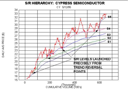
By way of example, consider the Midas chart (obv omitted to focus on
price alone) for Cypress
Semiconductor. Here we have a five-fold hierarchy of theoretical support
levels, where every member of the
hierarchy is launched precisely from a trend reversal point. Thus an
otherwise bewilderingly complex set of
zig-zags in the price history can be understood with respect to a single
algorithmic prescription: support will be
found at the volume-weighted average price taken over an interval
subsequent to a reversal in trend.
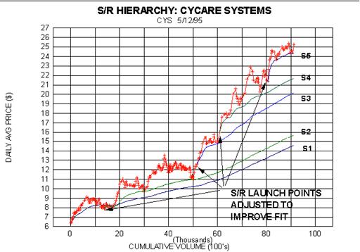
'Is this always the case?', one should now ask. In Count
Dracula's immortal words when his hapless
ovenight guests wished to leave: 'Ahh, if only life were so
simple!' Have a look at the Midas chart for Cycare
Systems. Here we could achieve a good 'fit' to the observed
price zig-zags only by adjusting the launch points
somewhat from their a priori values. In the case of S2, is was a matter
of determining where in the midst of an
extended consolidation bottom the launch point should taken. With S3 and
S4, it involved a displacement of a
day or two after the actual reversal day (a common situation in strongly
trending stocks). (S5 could be viewed
actually as an S6 - launched from the first pullback to an S5 which is
not shown.)
In all cases, we attempt to understand the actual price zig-zags within
a framework of the minimum
number of theoretical S/R's. The launch points for this minimal S/R
hierarchy are in the final analysis
empirically determined. However, in most cases, the initial guess of
launching the S/R's from the trend reversal
points is good enough.
Having thus developed the rationale for the Midas method of technical
analysis, we will henceforth get
down to the computational nitty gritty. After the next article (if not
by now) you should be generating your
own Midas charts and forming your own conclusions!
9
The previous two articles have described how one computes the hierarchy
of theoretical support/
resistance (S/R) levels upon which the MIDAS method of technical
analysis is based. This description has
intentionally avoided mathematical detail in order to focus on the
conceptual foundations. We now turn to the
actual equations and show how they can be readily evaluated in a
spreadsheet.
Suppose the input data spans a consecutive period of N days. On any
given day, say the i-th, we denote
the high, low and volume as H(i), L(i) and V(i) respectively. These are
the data that are actually used by MIDAS;
we do not require the open, close or calendar date. (If the available
input data only gives a single price - the
close for example - then simply set the high and low equal to this
price; if volume data is not available, set the
volume for every day equal to the same value - say one share. Having
less than complete input data is less than
ideal but not a fatal drawback).
The first step is to compute for each day the average price P(i):
P(i) = .5*( H(i) + L(i) )
Next, compute the cumulative volume for the i-th day, cumvol(i):
cumvol(i) = cumvol(i-1) + V(i)
That is we simply add the new day's volume to the cumulative volume at
the previous day. To start this
process, we set the cumulative volume initially to zero so that at the
end of the first day cumvol(1) = V(1).
In a similar fashion, also compute the cumulative product of the daily
price and daily volume. Calling this
cumpvol(i), we have
cumpvol(i) = cumpvol(i-1) + P(i)*V(i)
Again we start cumpvol at zero, so that at the end of the first day
cumpvol(1) = P(1)*V(1).
Finally, the on-balance volume for the i-th day, obv(i), is computed
from the equation
obv(i) = obv(i-1) +sgn(i)*V(i)
where the 'sign' function, sgn(i), is defined by
sgn(i) = +1 if P(i) > P(i-1)
sgn(i) = -1 if P(i)
< P(i-1)
sgn(i) = 0 if P(i) = P(i-1)
We arbitrarily choose sgn(1)=1 on the first day so that obv(1)=V(1).
The MIDAS chart is then constructed by plotting two separate (i.e. non-overlapping)
graphs, one placed
vertically above the other so that their x-axes are parallel. In the
upper graph, plot P(i) as the y- coordinate
versus cumvol(i) as the x coordinate. In the lower graph, use the same x
coordinate (i.e. cumvol(i) ) and plot
obv(i) as the y coordinate. Thus every day gives rise to a single x-y
point in each of the two graphs. Connecting
the sequential points in each graph thereby traces out curves of price
vs. cumulative volume in the upper graph
and on-balance volume vs. cumulative volume in the lower graph.
The last step is to plot the theoretical S/R curves on the same graph
that has price vs. cumulative
volume. The equation for computing the value on the i-th day of an S/R
level 'launched' on the j-th day ( call this
S/R(i , j) is simply:
S/R(i , j) = (
cumpvol(i) - cumpvol(j) ) / ( cumvol(i) - cumvol(j) )
That's all there is to it! One just interactively chooses a set of
launch points until an S/R hierarchy is (hopefully)
found which makes sense of the historical data, the initial launch point
guesses being the days of observed
reversals in trend.
An easy way of carrying out these calculations in practice is through
the use of a spreadsheet. Below I
show how this could be done in Lotus 123 (other spreadsheets will be
similar if not identical).
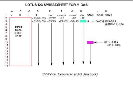
Simply enter the input data in the first three columns starting with the
second row, and enter the cell
formulas as shown in rows two and three. COPY the third row downward for
as many days (rows) as there
are input data. If an S/R level is to be launched from a given row - say
the 9-th - (e.g. because the value in the
'P' column reached a local maximum or minimum at that row)
then in the very next row (row 10) enter the
following formula in column I (the one labelled S/R#1):
+(F10 - F$9)/(G10 - G$9)
COPY it downwards to the last row of the data set. Note that the $ is
very important since it 'anchors' the
S/R level to the launch point (row 9 in the current example). Additional
S/R levels can be similarly launched in
columns J, K, etc. as the occasion demands.
Finally, using the graphing capabilities of the spreadsheet, create a
pair of x-y type graphs. In both
graphs, choose the x coordinate as the 'cumvol' column (G in
the present example). In one of the graphs, the
price vs. cumvol curve is generated by taking the y coordinate from the
'P' column (column D ) and the S/R
curve(s) from columns I (et al). In the other graph, take the y
coordinate from the 'obv' column (column H in the
figure).
From a practical standpoint, the time-consuming element is loading the
input data into the first three
columns. Those who are already using a spreadsheet to perform technical
analyses will presumably have
automated this process so the addition of MIDAS should present no
difficulties. Others may be using a
commercially available charting software package which both imports
historical data automatically and allows for
user-defined custom formulae or 'indicators'. In the next
article I will show how MIDAS can be integrated into
one such package.
POSTSCRIPT:
We are now approximately at the 'midterm' of what I view as a
course here at Cybercollege, one in
which you have enrolled by sticking with the articles to this point.
Your midterm 'exam' is simply to
provide me with some feedback: what you like and dislike about the
articles, any points you found unclear or
particularly enlightening, and in general any comments which may assist
me in making the remainder of the
course as useful as possible to you. On a personal level, a brief
biographical paragraph would also assist me in
visualizing the faces on the other side of my modem Thanks.
10
The tools have now been provided to analyze stock price behavior
relative to the theoretical hierarchy
of support/resistance (S/R) levels. How to use these tools to improve
one's trading performance -the
'engineering' aspect of MIDAS- is the focus of the present
article.
To paraphrase Hamlet, the basic question is 'to bounce or not to
bounce'. Our theory predicts where a
bounce (i.e. a trend reversal) should occur, and if it does occur, where
such a bounce should carry to as a
minimum objective. But, since the market is in the final analysis
probabilistic rather than deterministic, our
decision whether to trade an expected bounce - by buying at the
theoretical support and selling at a theoretical
resistance - will require some ancillary assessment of the likelihood
that the support level will in fact hold.
In the familiar and apt analogy between the stock market and the motion
of a cork floating on the sea,
one associates the broad tidal motion with the influence of the overall
market on a particular stock.
Superimposed on the tide are individual waves which are analagous to the
effect of the group (i.e. computers,
cyclicals, golds, etc.) to which the stock belongs. Finally there is the
microenvironment of ripples and wisps of
wind which relate to the particular dynamics of the stock itself.
Relegating to a later article the important topic of the application of
Midas methods to the overall
market, we look to the other two factors for the clues we seek.
Specifically, we can examine Midas charts
for two or more stocks in the same group on the assumption that one of
them will provide a leading indicator of
the group's behavior. Also, for a single stock we can consider the Midas
techniques in concert with other tools
from conventional technical analysis, seeking independent confirmation
that a tradable bounce may be at hand.
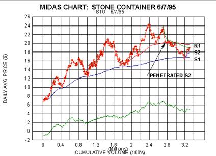
To pursue the group angle, we consider two paper product stocks:
Chesapeake Corp. and Stone
Container. The Midas chart for Stone Container updated to the time of
this writing is shown in the first figure.
The astute reader will recall that we visited STO before (in article
#2), at a time roughly corresponding to the tip
of the arrowhead in the figure. To recall our exact words: 'the
expectation is that the secondary (i.e. S2) will
hold and the price will resume its upward motion. If the secondary fails
to hold, the price would be expected to
decline at least to the primary support level at about 17.' In the
event, the secondary did hold for some time and
then ultimately failed after which support was found precisely at S1.
The subsequent bounce has carried to the
expected minimum objective, the resistance level R1, and at this moment
is attempting to penetrate it.
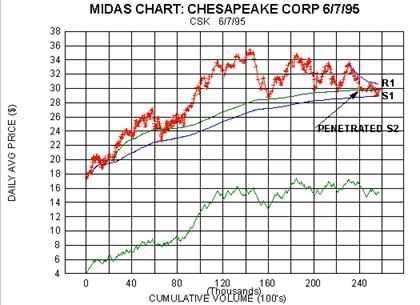
Now look at the Midas chart for Chesapeake Corp.Now look at the Midas
chart for Chesapeake Corp. As
with STO, the S2 support was penetrated after holding for some time, and
a bounce has started from the S1
level. It, however, has not yet carried as far as R1 and in this regard
is lagging behind STO. If STO in fact is
subsequently able to convincingly penetrate its R1, then this would give
incentive to buy CSK since the
implication is that the paper stocks have completed their correction and
are about to start a new bull leg.
Turning now to the concept of synergistically combining Midas methods
with other techniques of
technical analysis, this gives us an opportunity to redeem the promise
made at the end of the previous
article to show how Midas can be integrated into existing commercially
available charting software.
Windows on Wall Street (tm), a product of Market Arts Inc., is one such
package which automates the
importation of daily updates or historical stock data and allows the
user to produce charts incorporating a variety
of standard tools of technical analysis. As with other similar products
it also permits the introduction of
user-defined curves (or 'custom indicators') to be plotted on
the same graph as the price data. Unfortunately,
however, in common with all such packages (of which I'm aware) one is
limited to plotting vs time rather than vs
cumulative volume.
Nevertheless, it is quite simple to plot S/R levels using these
packages. In the case of Windows on Wall
Street, one merely defines the following 'custom indicator':
CUM(
.5*(H+L)*V*IF(CUM(1)>DAYS,1,0) ) / CUM( V*IF(CUM(1)>DAYS,1,0) )
where DAYS is a parameter equal to day (i.e. record) number at which the
S/R level is to be launched. (Defining
several such indicators, labelled S/R#1, S/R#2, etc, permits as many S/R
curves to be simiultaneously plotted
as one wishes). A particularly useful feature is that since DAYS is an
adjustable parameter, one can readily shift
the launch point around by simply clicking on the S/R curve with the
mouse, and then clicking on a
parameter-change button.
More importantly, one can combine on one graph other indicators and
technical aids together with the
Midas S/R levels. The third figure gives an example of this for Western
Digital (WDC). Here we have defined
three windows, one for an MACD histogram, one for on-balance volume, and
the main window for the price and
other technical aids. In addition to three Midas S/R levels, we have
included conventional trendlines (straight
lines joining peaks and troughs), so-called Bollinger Bands (2 standard
deviations above and below a moving
average of price), and bullish (green) and bearish (red) flags derived
from Japanese Candlestick pattern
recognition software.
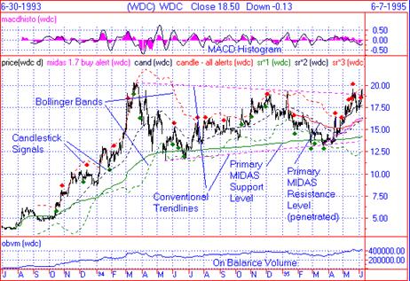
Focus particular attention on the March 1995 time frame. The price has
consolidated down to the primary
(S1) Midas support with a degree of porosity similar to the previous
contact (in May-June 1994). When the three
bullish candlestick signals appeared, this became a compelling buying
opportunity (especially the third such
signal at which time the price was simultaneously at both the trendline
and the lower Bollinger band).
The key to profitable trading using Midas is to have a sufficiently
large number of stocks under
surveillance, so that when such 'golden opportunities' come
along - as they surely do from time to time
- one can recognize them as such and concentrate enough buying power on
one's position to take full
advantage of the situation. This leads naturally to the question
'when should I sell?'. We'll discuss that in the
next article.
11
The insights into the underlying structure of price behavior provided by
Midas should be viewed as yet
another instrument in the toolbox of the technical analyst. By itself,
Midas is not the key to instant success
in trading; but when used skillfully in concert with other techniques
that one has already found to be useful, it can
provide the additional edge that is needed in what has become an
increasingly sophisticated and competitive
zero-sum game.
In the previous article, we have seen how intragroup comparisons and
synergistic use of other tools
can increase one's chances of identifying potentially profitable trend
reversals. (While we have
emphasized entry points for long positions, the inherent symmetry
between support and resistance hierarchies in
the Midas method allows the same methodology to be used in trading the
short side). Having thereby
determined 'when to buy', we raised the companion issue of
'when to sell'. In the course of examining this
question we will come to recognize some more fundamental structural
orderliness in price behavior - i.e. beyond
the mere existence of the S/R hierarchies.
In the early articles we have already cited some qualitative indications
that a bull move is running out of
steam: deterioration of the obv curve (i.e. obv starts to trend
downwards while the price is moving
sideways) or the appearance of fourth, fifth and even higher order S/R
levels. Now we know to watch out
also for bearish indications in the peer group of stocks, and for
ancillary signals such as trend line penetration,
classic chart reversal patterns (e.g. 'head and shoulders'), and
Japanese Candlestick alerts.
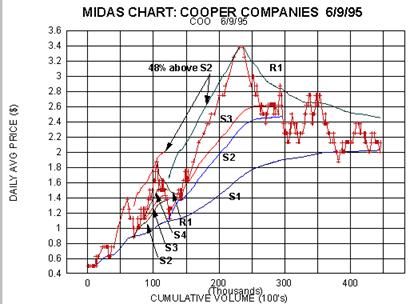
But does Midas itself have anything new to contribute in identifying
sell points? If one is trading a bounce
from a theoretical support level during a pullback from a recent high,
we have already seen many times that the
theoretical resistance level 'launched' at that high is a
viable price objective for the bounce. This is evident in the
Midas chart for Cooper Companies, for example, in the bounce from S2 to
R1 at a cumulative volume of about
290,000 (round lots).
I have chosen COO as an example because it has other lessons to teach.
Note the lines labelled '48%
above S2'. What we have done here is to ask the question 'how
high did the previous bull leg (the one peaking
near a cumulative volume = 100) go when expressed as a percentage above
its secondary support (S2)'? This
turned out to be 48%. We then apply the same percentage (what I call the
'greed factor') to the S2 for the next
leg to obtain a (moving) price target. Sure enough, the peak of the next
leg occurs where anticipated, although I
hasten to add that the agreement is seldom this precise!
We are exploiting the circumstance that successive bull moves are
frequently self-similar when viewed
in the context of the S/R hierarchy. Thus, if price excursions are
measured relative to the theoretical support
levels, different bull moves can be directly compared notwithstanding
the fact that they may occur over vastly
different scales of cumulative volume.
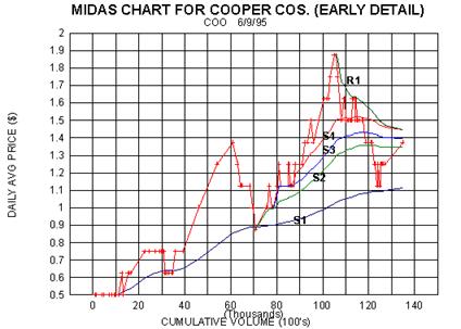
To pursue this point further, in the second figure we present a
magnified view of the bull move peaking
near cumvol=100. Plotted on the figure is a fourfold hierarchy of
support levels and the primary resistance level
launched at the peak. The important point to note is that although we
are only dealing with 54 days of data
(between cumvol= 70 and 125), there is nevertheless exhibited the same
hierarchal structure that one finds in
charts extending over several years. In other words, the zigzags in
price behavior that one observes on short
time scales have the same structure (in S/R hierarchal terms) as that
seen on long time scales.
The foregoing properties of self-similarity and scale independence are
characteristics of fractal
behavior. The fractal nature of stock price fluctuations has been
recognized for some time on purely empirical
grounds. What has been missing is an understanding of why markets should
behave fractallly (i.e. beyond the
obvious fact that they are complex non-linear dynamic systems). In the
Midas method, we have seen that the
complex zigzags in price behavior can be (to quote article#8)
'understood with respect to a single algorithmic
prescription: support (or resistance) will be found at the volume-
weighted average price taken over an interval
subsequent to a reversal in trend'. The psychological elements of
greed and fear, whose quantification led to
this algorithm, apply to investors/traders across all time scales.
(Someone who has held a stock at a loss for
three years is just as eager to 'get out even' as the day
trader who is holding a losing position).
There is even a more remarkable method of predicting tops (and bottoms)
in the Midas bag of tricks -
the so-called TOPFINDER algorithm. Don't miss the next article!
12
The truly new insights provided by the Midas method are twofold. The
first is the heretofore unrecognized
hierarchal structure of support/ resistance levels and their a priori
prediction in terms of the volume- weighted
average price taken over an interval subsequent to a trend reversal
point. The second, to be introduced in the
present article, is that there frequently exists a remarkable underlying
structure which dominates or 'guides' the
bull or bear move as it develops from that point onwards.
This structure is revealed when actual prices are compared to a new type
of theoretical
support/resistance curve generated by what I call the TOPFINDER
algorithm. (We expose our taurine - as
opposed to ursine - leanings as 'BOTTOMFINDER' would be
equally appropriate since the support/ resistance
symmetry applies to the new algorithm as well as the S/R hierarchy). In
presenting TOPFINDER, we will follow
the same pedagogical path used up to now. To whit, without initially
revealing the TOPFINDER equation, we will
show what are hopefully compelling demonstrations of its power. The next
steps in the program would then be
to outline the psychological principles underlying the mathematical
structure of the algorithm, followed by the
display of the algorithm itself.
In the present instance, however, the situation is reversed. I
discovered TOPFINDER empirically, and while
I have some ideas as to the underlying principles and mechanisms giving
rise to its applicability (which I will put
forth in due course), it is still a subject for conjecture and research.
Indeed, perhaps one of you will come up
with a useful approach!
To begin, then, let us turn to the figure wherein we revisit Union
Carbide. Recall from the fourth article that
following an extended period of 'foothill' behavior where UK
found repeated support at S2, it abruptly took off in
a doubling move during which support was found at successively higher
order levels - culminating with S5. In
time, this dramatic bull move ended and the price returned to the S3
level which was launched at the start of the
move.
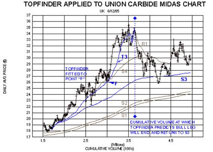
In the figure we show a new curve labelled 'T3', which is
launched concurrently with S3. As with the S/R
levels, this TOPFINDER curve is generated by a simple universal
algorithm , now containing two parameters to
be determined by fitting to the trend reversal points. As before the
first parameter is the launch point. In
TOPFINDER, the second parameter represents the duration of the move as
measured in cumulative volume.
In other words, TOPFINDER is predicting that the move which started with
the launch of S3 will, if the
move fulfils its 'destiny', terminate when the cumulative
volume reaches the value indicated by the
dashed line joining the diamonds, after which the price should return to
the more 'normal' (i.e.
unaccelerated) support S3. It is seen from the figure that if T3 is
fitted to the consolidation reversing at point
'F', then the end of the entire bull move is for all intents
and purposes predicted exactly!
Since technical analysis is often referred to these days as 'rocket
science', we can employ this
metaphor by likening a move in a stock to a rocket launch. Already we
have referred to a trend reversal as
the 'launch point'; now we imagine that - as with a rocket -
the move's duration is pre- programmed by loading a
given amount of 'fuel' which in our case is a fixed amount of
cumulative volume. During the powered phase of
the launch, the rocket's control mechanisms act to follow the nominal
trajectory defined by the TOPFINDER
curve. When the fuel is completely burnt, the rocket returns to the
Earth's surface represented by the S/R level.
In the market, as with rockets, there are abortive launches which do not
go all the way to burnout, but
return to Earth prematurely. Hence the TOPFINDER curve (and especially
the predicted burnout point) are to
be regarded only as potentialities. So the new viewpoint is that every
time there is a bounce from an S/R level of
order 'n', we begin the computation of two new curves: the
next higher- order S/R level (order 'n+1') and the
corresponding TOPFINDER labelled with the same index. The move
originating with the bounce has the potential
to 'take off' (i.e. accelerate) in which case its trajectory
is predicted by TOPFINDER. Or, it can fail to 'ignite' in
which case it merely rides along the newly launched S/R level in a
succession of less dramatic 'hops' before
either attempting a new takeoff- or penetrating the level and dropping
back down the hierarchy.
Returning to Union Carbide, I ask you - the jury - to disregard the dip
to the S3 level occurring at a
cumulative volume of about 2.6. (This was a one- day affair at the
climax of a 6-day 300 point drop in the
Dow in late March/ early April of 1994). With this point thus ignored,
it is seen that TOPFINDER - while explicitly
fitted to point 'F' - simultaneously does a good job of
accommodating all of the pullbacks from the start of the
move through the dip to 31 at a cumulative volume of about 3.3. (The
subsequent penetrations of the
TOPFINDER curve as the burnout point is approached are of no consequence
and a frequent occurrence for
reasons which will become clear when we exhibit the algorithm in a later
article). In this sense TOPFINDER may
truly be regarded as the guide curve for the entire price-doubling bull
move.
A second example - perhaps more striking in that no appeal to
forbearance is required - is afforded by
Borden Chemical and Plastics (BCU) in the second figure. Here the
TOPFINDER/BOTTOMFINDER
symmetry is explicitly exhibited. On the way up, TOPFINDER T3 accurately
locates the top of the accelerated
near- doubling move connected with the launch of S3, when fitted to the
first consolidation pattern. The
subsequent decline from the (triple) peak carries back to S3 as
expected, and even beyond to S2.
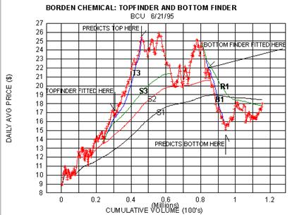
Later, after another rally to the area of the previous peak, BCU
undergoes a precipitous decline which is
well described by the BOTTOMFINDER curve B1, launched in conjunction
with the primary resistance
level R1. Again, when B1 is fitted to the first pullback, the cumulative
volume at which the bottom occurs is
accurately predicted. The subsequent pullback to R1 also exactly follows
the script.
It should be emphasized that applications of TOPFINDER (and
BOTTOMFINDER) are relatively
infrequent, yet quite striking when they do appear. Generally speaking,
whenever a bounce accelerates to
new highs before pulling back fully to the expected (i.e. newly
launched) S/R level, one should launch a
TOPFINDER, fitting it (provisionally) to the pull-back point. If the
move continues to trend strongly without
pullback to the S/R level, continue the TOPFINDER, perhaps iteratively
readjusting the fitting point as the move
matures towards the expected burnout cumulative volume.
Further examples of this remarkable new feature of price behavior will
be given in the article to follow,
after whiich we will present the underlying algorithm and speculations
as to its basis.
POSTSCRIPT:
In article#10, we gave a formula for introducing S/R's as custom
indicators in WIndows on Wall Street.
From readers' comments it is clear that I should have emphasized that
DAYS is a constant set by the user to
coincide with the launch point, being actually the number of records
from the beginning of the data file. One
reader, Stacie Crummie, discovered that with the following slight
modification (to avoid division by zero problems
prior to launch) , this formula can be used in the more popular
Metastock software:
cum(if(cum(1)<'days',0,mp()*v))/cum(if(cum(1)=1,1,if(cum(1)<'days',0,v)))
Here mp() is the mean price function, replacing our .5*(high+low).
Thanks Stacie.
13
In the previous article we introduced the concept of TOPFINDER (or
BOTTOMFINDER) wherein a
strongly trending move finds support (or resistance) on pullbacks at a
new type of S/R curve which
accelerates away from the normal S/R and terminates at a predetermined
cumulative volume. In order to
recognize the types of Midas curves for which TOPFINDER may be
applicable, it is worthwhile to examine a few
more examples before we present the algorithm and consider its
implications.
The first figure contains a Midas chart for a massive bull move and
subsequent bear correction in Swift
Transportation. In contrast to the Midas charts you have seen thus far
(which are generated by a Lotus 123
spreadsheet program I initially wrote for the HP 95LX pocket computer)
this figure is obtained from a Windows
application called WINMIDAS which we will discuss in a future article
(and possibly even have available for
download!).
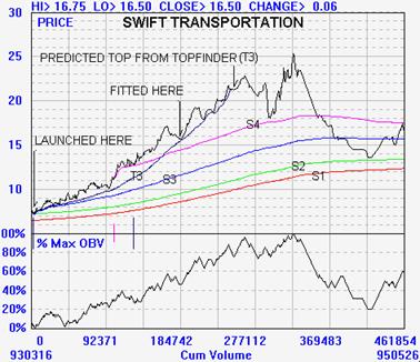
Per the comments in the previous article, after launching S3 and
observing that the price failed to pull
back to S3 - trending instead strongly upwards - a TOPFINDER curve T3
was launched as well. As the
move evolved, the point at which T3 was fitted to the various pullbacks
was refined until the final fitting point
shown in the figure was used.
Note that the subsequent pullbacks were well fitted by this TOPFINDER
curve but that the predicted
burnout was a bit premature. Furthermore, the subsequent correction went
only as far as S4, rather than S3.
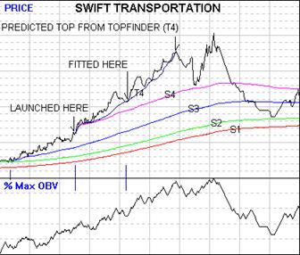
Was this a failure of the theory? Not quite, for (as shown in the second
figure) when we go back and launch the
TOPFINDER T4 associated with S4 - again fitting it to the same pullback
as with T3 - we find lo and behold that
with T4 the burnout point shifts to the right just enough to catch the
actual top!
So apparently just as there are short term bull moves contained within
longer term ones, TOPFINDERS
associated with different members of an S/R hierarchy can be
simultaneously operative. This is clearly
shown in the third figure which is an (older style) MIDAS chart for
Qualcomm (QCOM). Note first that the
TOPFINDER T1, associated with the primary support level S1, catches the
climax of the whole bull move quite
well (actually the first of the double-top formation).
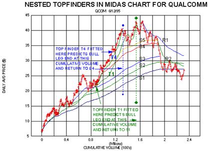
Yet within this 'six-bagger' move from 7 to 43, was a near
doubling move from about 22 to 41
associated with the launch of S4. If the corresponding T4 is plotted, it
is seen that the intermediate top is
located quite well when T4 is fitted to the short term pullbacks as
shown. (In the event, the subsequent
correction carried only to S5 rather than S4 as anticipated, but this
deviation from form could be interpreted as a
complication arising from the fact that the T1 had enough
'fuel' left to counteract the decline from the T4 peak.)
The foregoing examples underscore the circumstance that application of
TOPFINDER techniques
frequently involve ambiguities either in the choice of launch and
'fit' points, or in the possibility for
more complex simultaneous structures. While a regrettable frustration in
our search for the magic wand that
turns all to gold, there do occur 'textbook' examples devoid
of such complications which have great profit
potential.
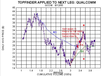
So to end on this positive note, let's go a bit further with QCOM and
look at the next bull leg - another
double from 16 to 32. As seen in the fourth figure, the straightforward
T1 associated with the new S1 works
like a charm catching the top exactly. So something is clearly going on
here and in the next article we'll examine
the TOPFINDER algorithm and try to understand why it works.
14
Strongly trending price moves are distinguished by their motion away
from the theoretical S/R level
launched at the start of the move. In several examples we have seen how
these accelerated moves find
support (resistance) at a TOPFINDER (BOTTOMFINDER) curve which
frequently has the ability to predict the
cumulative volume at which the move will end. In this article we present
the TOPFINDER algorithm and discuss
its implications.
To understand TOPFINDER, it is worthwhile to rewrite slightly the
algorithm used to generate the S/R
levels. In the first figure we collect all of the MIDAS algorithms,
written in their most useful form. The S/R levels
are given by the quantity called 'P-Bar-Star', where P stands
for price, Bar for average, and Star being an
acronym for 'subsequent to a reversal'. By this device, the
symbol itself - when given its mathematical
pronunciation - describes how it is to be computed (the average price
subsequent to a reversal)!
From the equation for P-Bar-Star, it is seen that it is now expressed in
terms of the cumulative volume
difference (or 'displacement' as we shall call it) between the
launch point and the point of computation.
The S/R level is simply the cumulative price*volume at the given instant
minus the cumulative price*volume at a
point d units of cumulative volume earlier, all divided by d, where d is
the displacement measured from the
(fixed) launch point.
We now define a new quantity called 'P-Hat', where
'Hat' is now an acronym for 'hitting a top'. P-Hat is
the TOPFINDER (or BOTTOMFINDER) curve, and is computed by an equation
which looks very much like that
for P-Bar-Star. The difference lies in the relationship between the
effective displacement, e, used in the P-Hat
equation and the displacement, d, used in the P-Bar-Star equation.
Specifically, e is related to d parabolically
through the equation e=d*(1-d/D). D is now a new parameter which we
shall call the 'duration' of the move since
e goes to zero when d approaches D.
The TOPFINDER algorithm (i.e. the equation for P-Hat) simply says that
instead of keeping the launch
point fixed (as with P-Bar-Star) one allows it to move forward in time
towards the present. In effect the
launch point can be visualized as chasing the present, finally catching
up when the D units of cumulative volume
have built up subsequent to the starting launch point. Putting it
another way, as the move uses up its allotted
duration, the topfinder curve represents an average price taken over
successively shorter intervals, whereas the
S/R level is an average taken over successively longer intervals.
This is illustrated in the second figure which shows the relationship
between e and d. We have drawn the
actual parabolic curve for e, as well as three linear tangents and their
corresponding cumulative volume 'zones'
I,II, and III. In zone I, the start of the move, e and d are very close
to each other so the topfinder launch point,
while actually moving away from the starting launch point, doesn't move
very far. The TOPFINDER and S/R
urves are thus close to one another in this initial zone. (Indeed, it is
the failure of the price to pull back fully to the
S/R curve, that alerts us to the fact that topfinder is coming into play
since a shorter displacement than d is
required to 'fit' the actual price pullback).
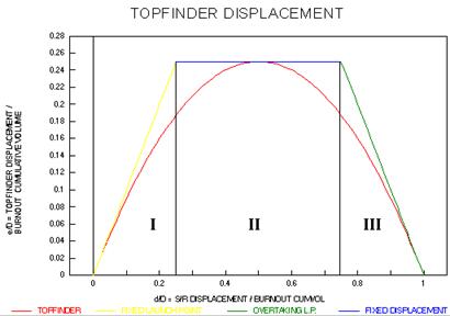
In zone II, the topfinder displacement is roughly constant at a value
close to one-quarter of the duration
D. If D were 100,000 shares, for example, then in zone II the price is
finding support (or resistance) at a price
average taken over the past 25,000 shares. This is behaving, in effect,
like a conventional moving average,
taken over a fixed number of shares rather than a fixed number of days.
In zone III, the effective displacement is rapidly diminishing. In fact,
to a first approximation, for every new
share traded while in this zone, the averaging interval shortens by one
share. It is this remarkable feature of the
climactic end of the move that gives us a clue as to what might be going
on.
Let me describe one situation which would lead to this type of behavior.
Forget for the moment that we
are discussing stocks or commodities and imagine that you are a dealer
in collectibles (coins, fine art,
etc.) You decide that, say, snuff boxes which are now in very little
demand could be promoted into a fashionable
collectible. So what do you do? First, very quietly so as not to tip
your hand, you start buying up all the snuff
boxes that come on the market. This is zone I, where if you recall the
psychology of the 'accumulator' described
in article #7, the price finds support at an S/R level. When you have
finally accumulated your desired level of
inventory, you start promoting snuff boxes as a collectible thereby
creating demand in the general public. You
sell your inventory at retail and - deciding that the demand for snuff
boxes will continue to be strong for some
time - you replenish your inventory by buying at wholesale as the
ever-present traders who have jumped on the
snuff-box bandwagon take their profits. This all takes place in zone II,
which we may call the 'trading zone',
where the fixed inventory is turned over by changing hands within a
group of trend following traders (of which
you are the leader by virtue of your preeminent position). Finally, you
observe that the number of snuff boxes
coming up for sale is diminishing because they are moving into weak
hands who are putting them away in vaults
for the long term. This decreased liquidity in the market means that you
will not be able to make as much as a
trader since the turnover will be diminishing. You therefore decide to
liquidate your remaining inventory and go on
to something else. In this 'distribution phase' (zone III),
you support the market as required by buying on
pullbacks in order that the price shall continue upward to attract the
remaining johnny-come-latelys to buy the
last of your inventory at the top of the market. Thereafter, you no
longer have any interest in supporting the price
and it drops of its own weight as few buyers are now found to maintain
an orderly market.
This'accumulation-trading-distribution' sequence involving a
fixed number of shares or contracts can
arise in a number of different ways. One is a direct analog of the above
scenario where - through skillful hype
- stocks are cynically promoted to unrealistic valuations and foisted
upon an unsuspecting public. On a more
refined - though no less cynical - level, corporate insiders wishing to
sell a large block of their stock engage an
investment banker to optimally distribute this block, who then through
'road shows' and the like beats the drum
for the institutional buyers always looking for a new
'concept' . Other scenarios can no doubt be conceived (eg.
short squeezes), wherein a specific number of shares are involved in a
dynamic process significantly different
from the normal ebb and flow of supply and demand, and where the normal
dynamics are restored when such
shares have been absorbed. Why the specific parabolic formula for the
effective displacement should work so
well remains an interesting question in search of a viable model.
(Analogs to the 'two-fluid' models of low
temperature physics come immediately to mind).
The actual computation of P-Hat from the above equation requires some
discussion which will be given
in the article to follow. There, we will also give examples of stocks
which are presently following topfinder
curves, so that testable predictions of future tops can be made.
15
The TOPFINDER algorithm given in the previous article has been seen to
be useful in 'predicting' tops
in historical price data. As the saying goes: 'Prophecy is
extremely difficult, especially as regards the future!'.
So in the present article we will apply TOPFINDER to a few stocks which
have not yet reached their peaks. The
future price action in these issues will thereby provide demonstrations
of either the power or the limitations of the
method.
First, however, a few words are required regarding the mechanics of
applying the TOPFINDER
algorithm. First one must pick a launch point, i, which identifies the
day on which TOPFINDER is to start. Also
the duration, D, must be chosen, where D is the cumulative volume from
the launch point to the top. D is actually
determined by iteratively adjusting it to provide a best 'fit'
to the price pullbacks subsequent to launch. To start
this process, one must set D equal to some initial guess; I usually
choose fifty days worth of volume, i.e. the
cumulative volume at launch minus the cumulative volume fifty trading
days earlier. In the fitting process used to
determine D, generally an 'eyeball' affair, give more weight
to fitting the more recent pullbacks.
The actual computation of the TOPFINDER curve involves interpolation
since we compute the
difference between the current value of cum(p*v) and the corresponding
value e units of cumulative
volume earlier where e = d*(1 - d/D). 'd' is the cumulative
volume at the day for which the TOPFINDER curve
is being computed minus the cumulative volume at lauch. e, therefore,
will generally fall in the middle of some
trading day so one has to interpolate linearly between the average price
at the close of that day and the average
price at the close of the preceding day.
In other words, cum(p*v) is only available from the data at a set of
discrete cumulative volumes
corresponding to the end of each trading day. Yet we are treating
cum(p*v) as a continuous function of
cumulative volume in order to determine it at values of cum(v) which do
not generally correspond to one of these
discrete points, and for this purpose we interpolate between the
discrete values of cumulative volume bracketing
e. Computationally, this will generally require a macro in a spreadsheet
implementation of Midas, or some simple
interpolation procedure if a high level language is used. Here I'll have
to leave you to your own devices since to
help you set up such calculations would carry us beyond the scope of
these articles.
Turning now to prophecy, the first figure shows TOPFINDER applied to LSI
Logic as of the day of
writing this article. (obv has been omitted from the Midas chart so we
can show more details of the price
data). Shown are the primary support S1 (unlabelled for simplicity), and
two TOPFINDER curves, labelled T1
and T2. T1 is launched at cum volume=0, and thus is the topfinder
counterpart of S1. T2, on the other hand is
launched at the point (cumvol around 2.5 million) where the price takes
off from the primary and where we
ordinarily would therefore start S2. (Again to keep the graphics simple,
I have omitted S2).
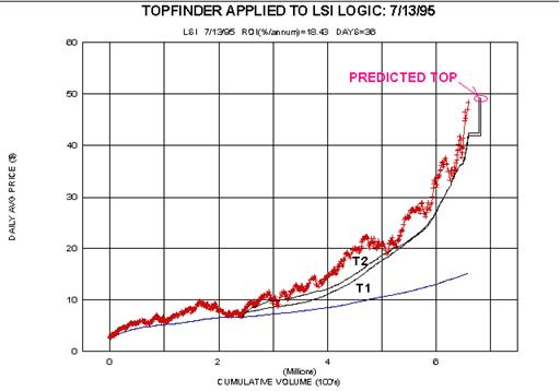
Each TOPFINDER curve terminates in a backward 'L' representing
the extrapolation of the curve to the
predicted top. The horizontal line shows how much cumulative volume is
left until the top, while the vertical line
terminates in a price projection determined by a simple linear
extrapolation of the tangent to the topfinder curve
at the endpoint of the data set. Recalling that TOPFINDER actually
predicts the cumulative volume at which the
price should top out, rather than the price itself, it should be borne
in mind that the predicted topping price is only
an extrapolated estimate, whereas the cum vol is the firm prediction.
I have included two topfinder curves in order to explore the sensitivity
of the predicted top to choice of
launch point. In each case, I did an independent eyeball fit to the
pullbacks subsequent to launch. Thus, T2
tries to fit the minor pullbacks around cumvol=3.5 million, whereas T1
tries to fit the main pullback points starting
at cumvol=3 million. It is quite remarkable that a single value of D can
do so well in each case, and it is gratifying
that the two agree so closely in their predictions of the top. (By
dividing the predicted cumulative volume left to
go by the average daily volume during the past fifty days, we arrive at
an estimate of 36 trading days to the
top).
While the LSI Midas graph was generated by a Lotus 123 spreadsheet
macro, the second figure - for
EMC Corp - was produced by a Windows application called WINMIDAS. This
software, written by my
colleague Dr. Stokes Fishburne, performs the topfinder and S/R
computations 'on the fly' in C++, so that one is
able to move the launch points and adjust D by simply clicking and
dragging the mouse - with the S and T curves
instantly adjusting to these changes!
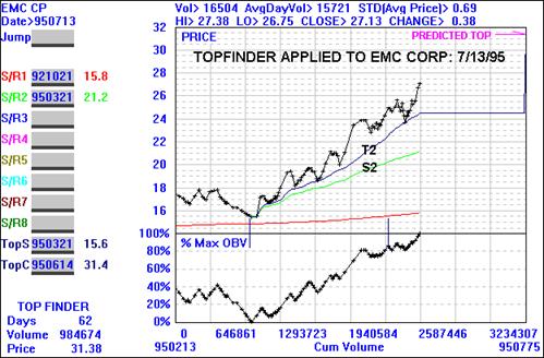
We have seen EMC before in article #5, which was written just after the
launch of S2 in the current
figure (labelled S3 in the earlier article). The failure of the price to
pullback to S2 was the clue to try
TOPFINDER and it is seen that T2 fits all the pullbacks quite well. As
indicated in the lower left hand corner of
the figure, the cumulative volume left to go is predicted to be 984, 674
round lots or 98,467,400 shares - about
62 trading days worth at the current level of activity. The extrapolated
price at the top is 31 3/8. If EMC follows
this script, then we would expect a pullback to S2 which, at that point
would be in the 22-23 range.
Having thus ventured into the future on a few individual stocks, in the
article to follow we see what
happens when we apply TOPFINDER to broad market indices like the S&P
500 and the Dow 30 - a topic
of particular interest since the predicted tops are imminent!
POSTSCRIPT:
The above article was written on July 13, 1995; it is now July 29th. The
intervening 16 days have included
the sharp (130 Dow points) selloff of July 19th in which the
'tech' stocks were particularly hard hit.It is
interesting to see how TOPFINDER fared in the face of this selloff for
our examples (LSI and EMC - both tech
stocks).
There are, in general, three possible outcomes of a market sell-off on
TOPFINDER. Usually, the effect is
to shift the top further into the future, readjusting as it were the
constant D to accommodate a pullback deeper
than had been anticipated. (One may use the analogy of a minor
earthquake which has the effect of releasing
some of the pent-up stresses thereby buying some additional time before
the 'big one' hits).
Alternatively, the trauma may be sufficiently severe to abort the
'launch' entirely - in the rocket metaphor of
article #12. This is what happened with EMC. As seen in the third
figure, the price pulled back exactly to 'earth'
(S2) as anticipated.
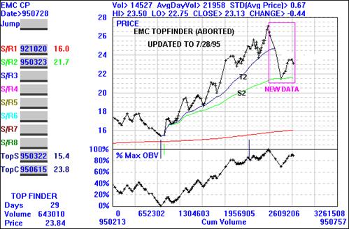
Or, TOPFINDER can take the selloff in stride. This may be what is
happening with LSI. As seen in the fourth
figure, the current price is quite close to the predicted top although
some volume remains before burnout. To be
sure, the pullback did penetrate the TOPFINDER curve somewhat (as would
have been evident if we had
updated it) and some readjustment of D may have been in order. For the
present, the jury is still out but a verdict
will be forthcoming shortly. In either event, it is quite often the case
- as it is here - that TOPFINDER provides
remarkably accurate price projections even if the top should turn out to
occur later than anticipated.
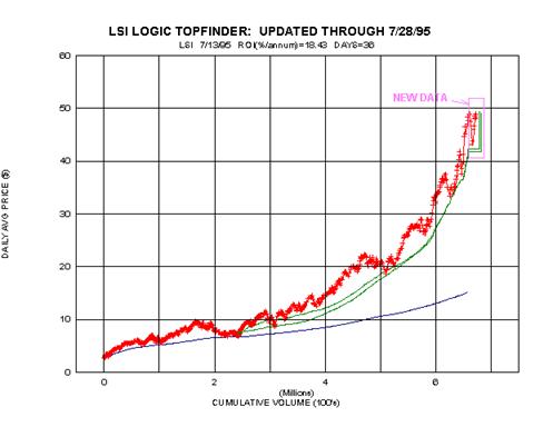
16
We have thus far applied the MIDAS method of technical analysis to
individual stocks, although we
speculated at the outset that its applicability extended to markets in
general. To the extent that all
markets are driven by the same basic psychological factors, this is
perhaps not too unreasonable an idea. In the
few remaining articles of this series, we will therefore look at some
new types of market data from the MIDAS
perspective. We begin here with stock market indices.
Market indices are simply the weighted averages of the prices in a subset
of the universe of stocks. The
'Dow' (Dow Jones Industrial Average) uses thirty high
capitalization companies at the core of the American
economy. The S&P-500 is based on a broad cross section of medium to
high capitalization companies spanning
the whole range of economic activities. The NASDAQ Composite Index has
as its focus newer and more
dynamically changing enterprises. Each index thus represents a different
facet of the economy, or - more
properly - the consensus view or paradigm of the near to intermediate
term (6 months to a year) prospects
thereof.
Recalling our earlier analogy (cork floating on the ocean) that
individual stocks are strongly coupled to
the market 'tides', then one would expect that the zig zags in
market indices should parallel those seen
in individual issues. In filtering out the individual idiosyncrasies of
single stocks or stock groups, the indices
preserve the most basic aspects of the herd psychology, or as it's more
delicately phrased, the 'mood of the
market'. Since MIDAS tries to quantify this psychology, there is
hope that it will have some applicability.
Without further preamble, then, in the first figure we apply the full
MIDAS armamentarium to the Dow
from 1988 to the present. (We shall henceforth display only charts
generated by the WINMIDAS software,
since - captioning aside - the entire chart can be produced from scratch
in well under five minutes!) If we restrict
attention to the seven year period prior to December 1994, it is seen
the Dow was reasonably well
characterized by a three-tier hierarchy of MIDAS support levels, with a
pullback to S3 in mid December 1994.
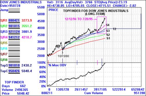
Furthermore, a TOPFINDER (T2) launched on 10/15/90 did a good job of
accommodating the three main
trend reversal points in that time period. The fact that this TOPFINDER
has about 662 trading days (about 2
1/2 calendar years) of 'fuel' left leads one to be generally
sanguine about the long term trend of the market and
- by implication - of the economy over this future span of time.
Since December of 1994, the market has taken off on an
uncharacteristically monotonic rise which has
every technician asking 'where will it end?'. Accordingly, in
the second chart we apply TOPFINDER to this
rise in the Dow. (To appropriately dovetail with the first chart, the
labels here should read S4 and T4 ). The chart
was generated on 7/13/95 and at that time we circled
('ellipsed' would be more appropriate) the fact that
TOPFINDER gave the market only two more trading days until a predicted
top of 4775 on July 17th.
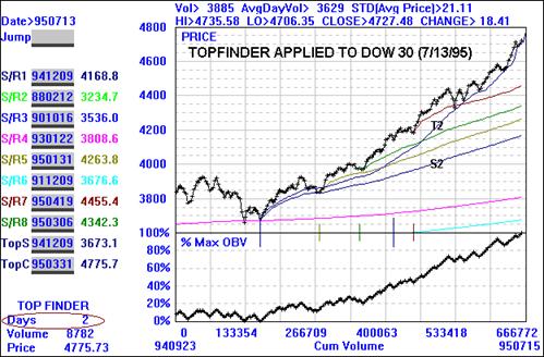
Ominously, when a corresponding MIDAS chart for the S&P 500 was
generated at the same time (see
the third figure), TOPFINDER predicted a top in this index as well two
days hence. As we shall see
presently, ditto for the NASDAQ. So we have the quite remarkable
circumstance that the same algorithm applied
to three distinctly different market indices was predicting a top at the
same time! (It must be freely admitted,
however, that prior to July 13th the ambiguities inherent in fitting a
two-parameter curve to rapidly rising price
data did lead to premature expectations of the top; however by July 13th
a sufficient number of zig zags were in
hand to define the TOPFINDER fairly unambiguously).
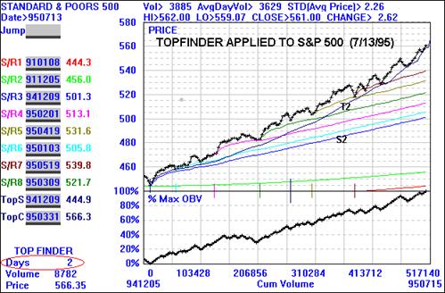
So what happened? On July 17th the Dow reached an intraday high of about
4770, and then proceeded to sell
off sharply in the next two days reaching an intraday low of about 4530
on Wednesday the 19th. 240 Dow points
top to bottom in two days! A triumph for TOPFINDER? Maybe, maybe not.
For as seen in the fourth figure
which is a MIDAS chart for the NASDAQ Composite Index, generated after
the close on July 28th, the sharp
drop subsequently reversed itself and we are now back to where we were
on July 17th (in fact slightly higher).
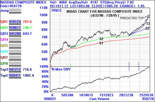
The ultimate verdict on TOPFINDER's utility in timing the market is
therefore still with the jury. If the
market henceforth extends its gains over a time span of more than a few
weeks (which we could view as a
reasonable margin of error in top prediction) then the only conclusion
that can be reached is that TOPFINDER
by itself (i.e. without the use of supplementary indicators) is not a
reliable timing tool for market indices. My
suspicion is, however, that TOPFINDER does have some truth in it.
Perhaps it catches the top of the left
shoulder in a head and shoulders top, or the first top in a double or
triple top formation. Or maybe in this case at
least MIDAS has come up with 'fool's gold'! Time will tell.
TOPFINDER aside, the MIDAS S/R hierarchy does in fact appear to be
useful in characterizing trend
reversal points in market indices, as was seen in the first figure. At
the very least, it provides downside
targets (i.e. expected points of at least temporary support) in any
selloff which might materialize. If the market
should appear to be bouncing from such a theoretically predicted level
one would take such a bounce seriously.
Thus MIDAS can be viewed as an otherwise unavailable filter for deciding
whether a given bounce is tradable or
of the 'dead cat' variety.
In the next article we will look at commodities and foreign markets.
17
The previous article has demonstrated the applicability of the MIDAS
techniques to stock indices based
on the US market. While some questions remain concerning the reliability
of TOPFINDER in such cases, it
appears that the S/R hierarchy has value in the characterization of
these indices. An interesting question, to
which we turn in the present article, is whether indices based on other
markets are similarly amenable to MIDAS
methods.
There is a lively contemporary interest in overseas stock markets, a
trend that can only accelerate in
the years to come. If MIDAS can be applied to such markets, the universe
of potential trading opportunities will
at least double so this is an important question for the MIDAS trader.
Accordingly, in the first figure we examine
the Hong Kong Hang Seng Index for the time period from 12/19/94 through
6/23/95.
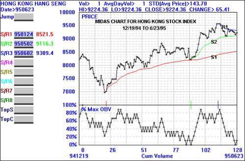
It is immediately evident that the S/R hierarchy is alive and well in
the Crown Colony! A 'text book case' if
there ever was one: well validated (i.e. non-porous) primary and
secondary support levels launched precisely
from the trend reversal points, and a classic 'squeeze'
between the secondary support and the primary
resistance levels. OBV is seen to be of little value, however, since
volume data was not available and thus OBV
counts only up days minus down days, rather than money flows in and out.
The precision of the S/R levels is all
the more remarkable since they were constructed in the absence of volume
data, viz. by assigning equal volume
to each day. (In the days subsequent to June 23rd, the squeeze was
resolved to the upside with penetration of
R1 and new highs for the index, followed by a retreat back to and bounce
from S2).
Even more impressive is the application of MIDAS to the Sydney All
Ordinaries Index of Australian
stocks shown in the second figure. Here, again notwithstanding the lack
of volume data, a four-fold hierarchy
of support levels - each launched precisely from a trend reversal point
- exactly fits the zig zags in the index.
(Again OBV is of no apparent value). Since there are many ways to
'play' the Australian market, from single
country mutual funds to the ADR's of Aussie companies, this may prove to
be a lucrative arena for MIDAS
traders.
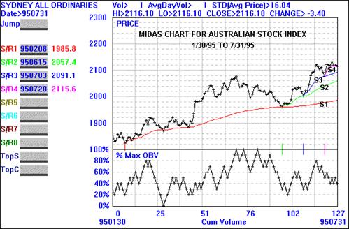
In terms of sheer dollar volume, the foreign exchange markets dwarf the
equities markets and it is
therefore understandable that the forex trading desks are the Cape
Canaveral of the 'rocket scientists'.
Does MIDAS have anything to contribute to this arena? The third figure
is a longer term chart of the US Dollar
Index from 11/24/93 to 6/23/95. While not as perfectly clean as the
first two examples, the four-fold hierarchy of
resistance levels would clearly have proven of value in predicting trend
reversal points. Furthermore, OBV being
meaningful in this case, there is no question - from the MIDAS
standpoint - of the intrinsically weak long-term
technical position of the dollar. From a shorter-term currency trading
standpoint, the position of the resistance
levels (updated, of course, to the present time) would provide price
objectives for the quick snap-back type
rallies often seen in long-term downtrends.
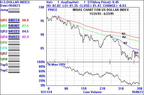
Finally, in the fourth figure we turn to commodities - specifically the
Commodity Research Bureau Index
which is a weighted average of the dollar price of a basket of diverse
commodities. As such, it reflects
both currency swings as well as the averaged effects of cyclical and
commodity-specific supply/demand
imbalances. It is therefore no surprise that the data is noisier than we
have heretofore seen. Nevertheless, there
is no question in the mind of the MIDAS theorist that a trend change has
occurred (R1 penetrated, OBV at new
highs), nor is there any uncertainty as to where to expect a bounce in
the next decline (S2). (In point of fact, the
next pullback on July 10th came to within a half-point in average price
to S2).
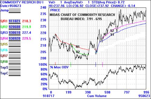
The whole commodities arena (indices, spot and futures) is terra
incognita as far as MIDAS applications
are concerned. My very preliminary research indicates that MIDAS
techniques can provide trading advantages
only on relatively short time scales (a few weeks) and only on some
commodities at some times. In other words,
when it works it works and carpe diem is the dictum.
Having thus exhausted both my Latin and the findings of several decades
of MIDAS research, we have
clearly reached a natural boundary in this Introductory exposition. In
the final article of the series, we will
provide a dramatic recapitulation of the MIDAS method, and some
valedictory remarks.
18
The goal of technical analysis is to discern underlying patterns of
orderliness in the apparent random
walk of prices and to use such perceived structures as the basis for
projections into the future of past
price behavior. The ever-present danger in this endeavor is one of
self-delusion: seeing patterns where none
really exist and - worse yet - trying to use such patterns to predict
the unpredictable.
It was therefore particularly gratifying that the search for a final
example on which to base our
concluding remarks uncovered the long-term MIDAS chart for AT&T
shown in the figure. Representing
eleven years of data, virtually every feature of the MIDAS method
detailed in the foregoing articles is exemplified
in this single chart.
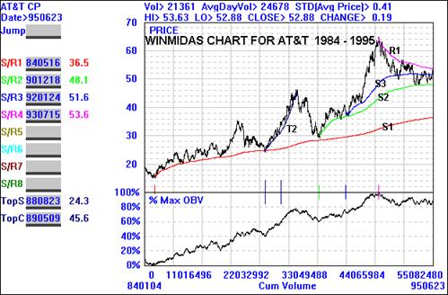
First, one can only marvel that the primary support level, S1, nearly
precisely coincided with seven
points of trend reversal over the six-year period 1984 - 1990.
Similarly, the secondary support level, S2,
launched in December 1990 has precisely accommodated at least a half-
dozen trend reversals with negligible
porosity. The primary resistance level, R1, is similarly validated and -
together with S2 - has the price trapped in
a classic 'squeeze' pattern. The tertiary support S3 has
functioned as a resistance level after having been
penetrated. Early in the chart, the foothill behavior is quite evident
and even TOPFINDER makes its appearance
in the near-doubling move from the mid-twenties to the mid-forties!
Finally, the fractal character of the S/R
hierarchy is clearly demonstrated since this eleven year MIDAS chart is
indistinguishable in its morphology from
the many year-long charts we have seen in the various articles.
So it seems clear that MIDAS is for real and has much to contribute to
technical analysis; self-delusion
does not seem to be a problem. Consider the richness of detail and the
ease of interpretation which MIDAS
provides. A single glance at the chart shows immediately that AT&T
is involved in a silent combat between S2
and R1. Failure of S2, i.e. resolution of the squeeze to the downside,
means a retreat to S1 at about 37 (and a
great buying opportunity at the first sign of a bounce there). A
convincing penetration of R1, on the other hand,
implies at least a retest of the previous high. By way of comparison,
some one looking at the conventional
price-volume bar chart for the past year shown in the second figure
would probably conclude that here is
another example of random walk behavior!
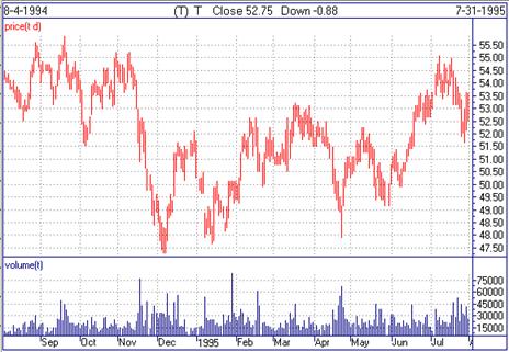
Thus, just as we began this series of articles with a side by side
comparison of a MIDAS chart and a
conventional bar chart, so shall we conclude this informal monograph.
Those who would integrate these
techniques into their trading discipline are advised to be ever mindful
of the fact that the market is in the final
analysis inherently unpredictable. All MIDAS does is to define more
clearly the tracks along which the market
has been moving and - absent shocks and paradigm shifts - will
presumably continue to move. As powerful as
the MIDAS techniques appear to be, they will frequently be humbled by
the market's caprice. Just as King Midas
found to his grief, power always has its limitations, often from the
least expected quarter.
Finally, this is a good opportunity to address two of the most
frequently asked questions in the
correspondence provoked by these articles. First, 'Does MIdas work
for every stock?' Midas works best
when a stock is in a coherent trend. Some stocks at some times are not
and are better described in terms of a
random walk. As an informal estimate based on years of experience, I
would guess that at any given time, a
useful S/R hierarchy can be identified for about two out of three
stocks. TOPFINDER examples are generally
rare, perhaps of the order of one instance in a year's worth of data for
twenty stocks.
It has also often been asked 'Why are you disclosing these
techniques for free; why not try and sell
them in some form or other?' I have always felt that if MIDAS has
any practical value, ample rewards would
come from the market itself (and they have) far in excess of anything
that could be made from such
commercialization of the method. So long as MIDAS is not sufficiently
widespread that it becomes self defeating
as everyone is recognizing the same trading opportunities, there is no
reason not to share the insights with the
technical analysis community. It is my hope that the articles will
stimulate research along these new lines and
that the same spirit of openness will prevail in sharing the results.
