Use absolute references

use absolute references

As you saw earlier in this lesson, when you copy a formula, Excel tries to change the cell references so that they are appropriate to the new location. It does this whether you copy with AutoFill or using more traditional methods such as Copy and Paste.

Most of the time, this is a good thing. However, sometimes you might not want the cell references to change. For example, suppose you put the current interest rate in cell F1, and you want each formula in the worksheet to include it in its calculation. In a case like that, you would want F1 to remain F1 no matter where you copied the formula.

To 'lock' a reference so that it won't change when you copy it to another location, you use an absolute reference by adding a dollar sign ($) before the row and before the column. So, for example, F1 becomes $F$1. If you want to lock only the row, use the dollar sign only before the number, like this: F$1. To lock only the column, place the dollar sign only before the letter, like this: $F1.

Sounds pretty simple, doesn't it? Yet for some reason absolute references are difficult for many people to 'get' conceptually. Therefore, the rest of this lesson is devoted to giving you practice using these references.

If you want to follow along with the examples, enter the text and numbers shown in each figure and then follow the instructions.

example 1: interest rate

Let's start by doing a simple amortization table for a loan using an absolute reference.

1. Recreate the worksheet shown in Figure 3-3.

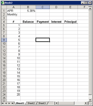
Figure 3-3: Use this data for the example.

2. In cell B2, enter =B1/12. This divides the annual percentage rate by 12 to produce the monthly interest rate.
3. In cell B5, enter the beginning balance for the loan. (We'll use $10,000 in this example, but you can use any amount you like. You also can change the annual percentage rate in cell B1 if you want to -- don't forget the percent sign.)
4. In cell C5, enter the amount you'll pay on the loan each month. For our example, we'll use $300.
5. In cell D5, enter =B5*$B$2. This multiplies the current balance by an absolute reference to B2.
6. In cell E5, enter =C5-D5. This deducts the interest paid from the amount of the payment; the result is the amount by which the principal should be reduced.
7. In cell B6, enter =B5-D5. This changes the balance by subtracting the principal paid in the previous month.
8. Copy the contents of D5:E5 down through D24:E24 using AutoFill.
9. Copy the content of C5 down through C24 using AutoFill. (You have to do this separately from Step 9, or AutoFill increments the payment, and you don't want that.)
10. Copy the content of B6 down through cell B24 using AutoFill.

Figure 3-4 shows the result.

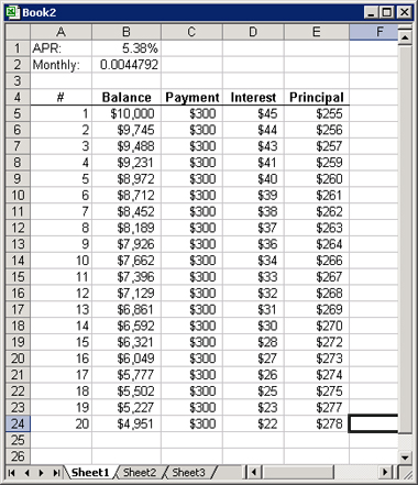
Figure 3-4: The finished example file.

Let's look at some more examples of using absolute references, because understanding them thoroughly is very important. By the time you're finished with this lesson and the assignment, you should understand them thoroughly.

example 2: sale prices

For this example, we look at how some prices are affected by a certain percentage of markdown at a retail store. Suppose you have been directed to create a price list for items that are going to be discounted for a sales event.

Start by reproducing the worksheet shown in Figure 3-5.

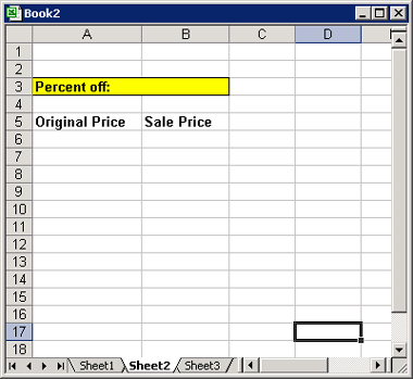
Figure 3-5: Start with this worksheet data.

1. In cells A6 and A7, respectively, enter $1.49 and
2. Select cells A6 and A7, and then fill the series down to cell A24. Cell A24 should show a price of $10.49.
3. In cell B3, enter the percentage off the regular price that you want to discount the items. For this example we use 25%. Don't forget the percent sign.
4. In cell B6, enter =A6-(A6*$B$3). This multiplies the original price by the percent off, and then subtracts it from the original price to determine the new price.
5. Copy the formula in B6 down through B24 with AutoFill. If you do it correctly, the sale price in B24 will be $7.87. Figure 3-6 shows the completed worksheet.

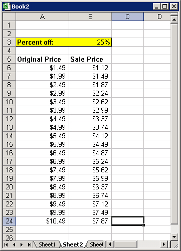
Figure 3-6: The finished example file.

example 3: investment income

If you place a certain sum of money today in a savings account, at a certain interest rate earned, how much will you have in 1 year, assuming interest is compounded weekly? In this final example, you answer that question.

Set up a worksheet that places the beginning balance and the interest rate in separate cells at the top. You'll refer to them in other formulas in the worksheet. Figure 3-7 shows one way to do it, but you'll need to figure out the formulas -- and which values should be absolute references -- on your own.

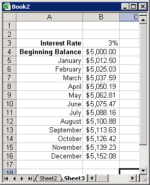
Figure 3-7: See if you can figure out the formulas to use for this worksheet to produce these results.