| CATEGORII DOCUMENTE |
| Bulgara | Ceha slovaca | Croata | Engleza | Estona | Finlandeza | Franceza |
| Germana | Italiana | Letona | Lituaniana | Maghiara | Olandeza | Poloneza |
| Sarba | Slovena | Spaniola | Suedeza | Turca | Ucraineana |
Predicting Protein Structure and Function from Sequence
The amino acid sequence of a protein contains interesting information in and of itself. A protein sequence can be compared and contrasted with the sequences of other proteins to establish its relationship, if any, to known protein families, and to provide information about the evolution of biochemical function. However, for the purpose of understanding protein function, the 3D structure of a protein is far more useful than its sequence.
The key property of proteins that allows them to perform a variety of biochemical functions is the sequence of amino acids in the protein chain, which somehow uniquely determines the 3D structure of the protein.[1] Given 20 amino acid possibilities, there are a vast number of ways they can be combined to make up even a short protein sequence, which means that given time, organisms can evolve proteins that carry out practically any imaginable purpose.
[1] That 'somehow,' incidentally, represents several decades of work by hundreds of researchers, on a fundamental question that remains open to this day.
Each time a particular protein chain is synthesized in the cell, it folds together so that each of the critical chemical groups for that particular protein's function is brought into a precise geometric arrangement. The fold assumed by a protein sequence doesn't vary. Every occurrence of that particular protein folds into exactly the same structure.
Despite this consistency on the part of proteins, no one has figured out how to accurately predict the 3D structure that a protein will fold into based on its sequence alone. Patterns are clearly present in the amino acid sequences of proteins, but those patterns are degenerate ; that is, more than one sequence can specify a particular type of fold. While there are thousands upon thousands of ways amino acids can combine to form a sequence of a particular length, the number of unique ways that a protein structure can organize itself seems to be much smaller. Only a few hundred unique protein folds have been observed in the Protein Data Bank. Proteins with almost completely nonhomologous sequences nonetheless fold into structures that are similar. And so, prediction of structure from sequence is a difficult problem.
10.1 Determining the Structures of Proteins
If we can experimentally determine the structures of proteins, and structure prediction is so hard, why bother with predicting structure at all? The answer is that solving protein structures is difficult, and there are many bottlenecks in the experimental process. Although the first protein structure was determined decades before the first DNA sequence, the protein structure database has grown far more slowly in the interim than the sequence database. There are now on the order of 10,000 protein structures in the PDB, and on the order of 10 million gene sequences in GenBank. Only about 3,000 unique protein structures have been solved (excluding structures of proteins that are more than 95% identical in sequence). Approximately 1,000 of these are from proteins that are substantially different from each other (no more than 25% identical in sequence).
10.1.1 Solving Protein Structures by X-ray Crystallography
In the late 1930s, it was already known that proteins were made up of amino acids, although it had not yet been proven that these components came together in a unique sequence. Linus Pauling and Robert Corey began to use x-ray crystallography to study the atomic structures of amino acids and peptides.
Pure proteins had been crystallized by the time that Pauling and Corey began their experiments. However, x-ray crystallography requires large, unflawed protein crystals, and the technology of protein purification and crystallization had not advanced to the point of producing useful crystals. What Pauling and Corey did discover in their studies of amino acids and peptides was that the peptide bond is flat and rigid, and that the carboxylic acid oxygen is almost always on the opposite side of the peptide bond as the amino hydrogen. (See the illustration of a peptide bond in Figure 9-1). Using this information to constrain their models, along with the atomic bond lengths and angles that they observed for amino acids, Pauling and Corey built structural models of polypeptide chains. As a result, they were able to propose two types of repetitive structure that occur in proteins: the alpha helix and the beta sheet, as shown previously in Chapter 9.
In experiments that began in the early 1950s, John Kendrew determined the structure of a protein called myoglobin, and Max Perutz determined the structure of a similar protein called hemoglobin. Both proteins are oxygen transporters, easily isolated in large quantities from blood and readily crystallized. Obtaining x-ray data of reasonably high quality and analyzing it without the aid of modern computers took several years. The structures of hemoglobin and myoglobin were found to be composed of high-density rods of the dimensions expected for Pauling's proposed alpha helix. Two years later, a much higher-quality crystallographic data set allowed the positions of 1200 of myoglobin's 1260 atoms to be determined exactly. The experiments of Kendrew and Perutz paved the way for x-ray crystallographic analysis of other proteins.
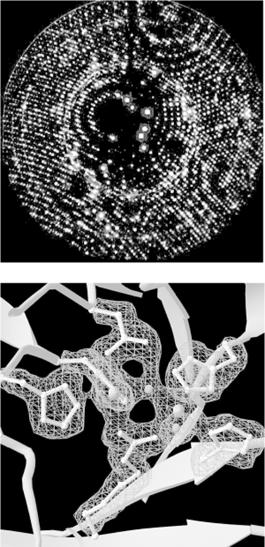
In x-ray crystallography, a crystal of a substance is placed in an x-ray beam. X-rays are reflected by the electron clouds surrounding the atoms in the crystal. In a protein crystal, individual protein molecules are arranged in a regular lattice, so x-rays are reflected by the crystal in regular patterns. The x-ray reflections scattered from a protein crystal can be analyzed to produce an electron density map of the protein (see Figure 10-1: images are courtesy of the Holden Group, University of Wisconsin, Madison, and Bruker Analytical X Ray Systems). Protein atomic coordinates are produced by modeling the best possible way for the atoms making up the known sequence of the protein to fit into this electron density. The fitting process isn't unambiguous; there are many incrementally different ways in which an atomic structure can be fit into an electron density map, and not all of them are chemically correct. A protein structure isn't an exact representation of the positions of atoms in the crystal; it's simply the model that best fits both the electron density map of the protein and the stereochemical constraints that govern protein structures.
Figure 10-1. X-ray diffraction pattern and corresponding electron density map of the 3D structure of zinc-containing phosphodiesterase
In order to determine a protein structure by x-ray crystallography, an extremely pure protein sample is needed. The protein sample has to form crystals that are relatively large (about 0.5 mm) and singular, without flaws. Producing large samples of pure protein has become easier with recombinant DNA technology. However, crystallizing proteins is still somewhat of an art form. There is no generic recipe for crystallization conditions (e.g., the salt content and pH of the protein solution) that cause proteins to crystallize rapidly, and even when the right solution conditions are found, it may take months for crystals of suitable size to form.
Many protein structures aren't amenable to crystallization at all. For instance, proteins that do their work in the cell membrane usually aren't soluble in water and tend to aggregate in solution, so it's difficult to solve the structures of membrane proteins by x-ray crystallography. Integral membrane proteins account for about 30% of the protein complement (proteome) of living things, and yet less than a dozen proteins of this type have been crystallized in a pure enough form for their structures to be solved at atomic resolution.
10.1.2 Solving Structures by NMR Spectroscopy
An increasing number of protein structures are being solved by nuclear magnetic resonance (NMR) spectroscopy. Figure 10-2 shows raw data from NMR spectroscopy. NMR detects atomic nuclei with nonzero spin; the signals produced by these nuclei are shifted in the magnetic field depending on their electronic environment. By interpreting the chemical shifts observed in the NMR spectrum of a molecule, distances between particular atoms in the molecule can be estimated. (The image in Figure 10-2 is courtesy of Clemens Anklin, Bruker Analytical X Ray Systems.)
Figure 10-2. NOESY (2D NMR) spectrum of lysozyme
To be studied using NMR, a protein needs to be small enough to rotate rapidly in solution (on the order of 30 kilodaltons in molecular weight), soluble at high concentrations, and stable at room temperature for time periods as long as several days.
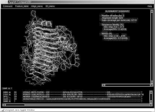
Analysis of the chemical shift data from an NMR experiment produces a set of distance constraints between labeled atoms in a protein. Solving an NMR structure means producing a model or set of models that manage to satisfy all the known distance constraints determined by the NMR experiment, as well as the general stereochemical constraints that govern protein structures. NMR models are often released in groups of 20 -40 models, because the solution to a structure determined by NMR is more ambiguous than the solution to a structure determined by crystallography. An NMR average structure is created by averaging such a group of models (Figure 10-3). Depending on how this averaging is done, stereochemical errors may be introduced into the resulting structure, so it's generally wise to check the quality of average structures before using them in modeling.
Figure 10-3. Structural diversity in a set of NMR models

10.2 Predicting the Structures of Proteins
Ideally, what we'd like to do in analyzing proteins is take the sequence of a protein, which is cheap to obtain experimentally, and predict the structure of the protein, which is expensive and sometimes impossible to determine experimentally. It would also be interesting to be able to accurately predict function from sequence, identify functional sites in uncharacterized 3D structures, and eventually, build designed proteinsmolecular machines that do whatever we need them to do. But without an understanding of how sequence determines structure, these other goals can't reliably be achieved.
There are two approaches in computational modeling of protein structure. The first is knowledge-based modeling. Knowledge-based methods employ parameters extracted from the database of existing structures to evaluate and optimize structures or predict structure from sequence (the protein structure prediction problem). The second approach is based on simulation of physical forces and molecular dynamics. Physicochemical simulations are often used to attempt to model how a protein folds into its compact, functional, native form from a nonfunctional, not-as-compact, denatured form (the protein folding problem). In this chapter we focus on knowledge-based protein structure prediction and analysis methods in which bioinformatics plays an important role.
Ab-initio protein structure prediction from protein sequence remains an unsolved problem in computational biology. Although many researchers have worked to develop methods for structure prediction, the only methods that produce a large number of successful 3D structure predictions are those based on sequence homology. If you have a protein sequence and you want to know its structure, you either need a homologous structure to use as a template for model-building, or you need to find a crystallographer who will collaborate with you to solve the structure experimentally.
The protein-structure community is addressing the database gap between sequence and structure in a couple of ways. Pilot projects in structural genomicsthe effort to experimentally solve all, or some large fraction of, the protein structures encoded by an entire genomeare underway at several institutions. However, these projects stand little chance of catching up to the sheer volume of sequence data that's being produced, at least in the near future.
10.2.1 CASP: The Search for the Holy Grail
In light of the database gap, computational structure prediction is a hot target. It's often been referred to as the 'holy grail' of computational biology; it's both an important goal and an elusive, perhaps impossible, goal. However, it's possible to track progress in the area of protein structure prediction in the literature and try out approaches that have shown partial success.
Every two years, structure prediction research groups compete in the Community Wide Experiment on the Critical Assessment of Techniques for Protein Structure Prediction (CASP, https://predictioncenter.llnl.gov/). The results of the CASP competition showcase the latest methods for protein-structure prediction. CASP has three areas of competition: homology modeling, threading, and ab initio prediction. In addition, CASP is a testing ground for new methods of evaluating the correctness of structure predictions.
Homology modeling focuses on the use of a structural template derived from known structures to build an all-atom model of a protein. The quality of CASP predictions in 1998 showed that structure prediction based on homology is very successful in producing reasonable models in any case in which a significantly homologous structure was available. The challenge for homology-based prediction, as for sequence alignment, is detecting meaningful sequence homology in the Twilight Zonebelow 25% sequence homology.
Threading methods take the amino acid sequence of an uncharacterized protein structure, rapidly compute models based on existing 3D structures, and then evaluate these models to determine how well the unknown amino acid 'fits' each template structure. All the threading methods reported in the most recent CASP competition produce accurate structural models in less than half of the cases in which they are applied. They are more successfully used to detect remote homologies that can't be detected by standard sequence alignment; if parts of a sequence fit a fold well, an alignment can generally be inferred, although there may not be enough information to build a complete model.
Ab-initio prediction methods focus on building structure with no prior information. While none of the ab-initio methods evaluated in CASP 3 produce accurate models with any reliability, a variety of methods are showing some promise in this area. One informatics-based strategy for structure prediction has been to develop representative libraries of short structural segments out of which structures can be built. Since structural 'words' that aren't in the library of segments are out of bounds, the structural space to be searched in model building is somewhat constrained. Another common ab-initio method is to use a reduced representation of the protein structure to simulate folding. In these methods, proteins can be represented as beads on a string. Each amino acid, or each fixed secondary structure unit in some approaches, becomes a bead with assigned properties that attract and repel other types of beads, and statistical mechanical simulation methods are used to search the conformational space available to the simplified model. These methods can be successful in identifying protein folds, even when the details of the structure can't be predicted.
10.3 From 3D to 1D
Proteins and DNA are, in reality, complicated chemical structures made up of thousands or even millions of atoms. Simulating such complicated structures explicitly isn't possible even with modern computers, so computational biologists use abstractions of proteins and DNA when developing analytical methods. The most commonly used abstraction of biological macromolecules is the single-letter sequence. However, reducing the information content of a complicated structure to a simple sequence code leaves behind valuable information.
The sequence analysis methods discussed in Chapter 7 and Chapter 8, treat proteins as strings of characters. For the purpose of sequence comparison, the character sequence of a protein is almost a sufficient representation of a protein structure. However, even the need for substitution matrices in scoring protein sequence alignments points to the more complicated chemical nature of proteins. Some amino acids are chemically similar to each other and likely to substitute for each other. Some are different. Some are large, and some are small. Some are polar; some are nonpolar. Substitution matrices are a simple, quantitative way to map amino acid property information onto a linear sequence. Asking no questions about the nature of the similarities, substitution matrices reflect the tendencies of one amino acid to substitute for another, but that is all.
However, each amino acid residue in a protein structure (or each base in a DNA or RNA structure, as we are beginning to learn) doesn't exist just within its sequence context. 1D information has not proven sufficient to show unambiguously how protein structure and function are determined from sequence. The 3D structural and chemical context of a residue contains many types of information.
Until quite recently, 3D information about protein structure was usually condensed into a more easily analyzable form via 3D-to-1D mapping. A property extracted from a database can be mapped, usually in the form of a numerical or alphabetic character score, to each residue in a sequence. Knowledge-based methods for secondary structure prediction were one of the first uses of 3D-to-1D mapping. By mapping secondary structure context onto sequence information as a propertyattaching a code representing 'helix,' 'sheet,' or 'coil' to each amino acida set of secondary structure propensities can be derived from the structure database and then used to predict the secondary structure content of new sequences.
What important properties does each amino acid in a protein sequence have, besides occurrence in a secondary structure? Some commonly used properties are solvent accessibility, acid/base properties, polarizability, nearest sequence neighbors, and nearest spatial neighbors. All these properties have something to do with intermolecular interactions, as discussed in Chapter 9.
10.4 Feature Detection in Protein Sequences
Protein sequence analysis is based to some extent on understanding the physicochemical properties of the chemical components of the protein chain, and to some extent on knowing the frequency of occurrence of particular amino acids in specific positions in protein structures and substructures. Although protein sequence-analysis tools operate on 1D sequence data, they contain implicit assumptions about how structural features map to sequence data. Before using these tools, it's best to know some protein biochemistry.
Features in protein sequences represent the details of the protein's function. These usually include sites of post-translational modifications and localization signals. Post-translational modifications are chemical changes made to the protein after it's transcribed from a messenger RNA. They include truncations of the protein (cleavages) and the addition of a chemical group to regulate the behavior of the protein (phosphorylation, glycosylation, and acetylation are common examples). Localization or targeting signals are used by the cell to ensure that proteins are in the right place at the right time. They include nuclear localization signals, ER targeting peptides, and transmembrane helices (which we saw in Chapter 9).
Protein sequence feature detection is often the first problem in computational biology tackled by molecular biologists. Unfortunately, the software tools used for feature detection aren't centrally located. They are scattered across the Web on personal or laboratory sites, and to find them you'll need to do some digging using your favorite search engine.
One collection of web-based resources for protein sequence feature detection is maintained at the Technical University of Denmark's Center for Biological Sequence Analysis Prediction Servers (https://www.cbs.dtu.dk/services/). This site provides access to server-based programs for finding (among other things) cleavage sites, glycosylation sites, and subcellular localization signals. These tools all work similarly; they search for simple sequence patterns, or profiles, that are known to be associated with various post-translational modifications. The programs have standardized interfaces and are straightforward to use: each has a submission form into which you paste your sequence of interest, and each returns an HTML page containing the results.
10.5 Secondary Structure Prediction
Secondary structure prediction is often regarded as a first step in predicting the structure of a protein. As with any prediction method, a healthy amount of skepticism should be employed in interpreting the output of these programs as actual predictions of secondary structure. By the same token, secondary structure predictions can help you analyze and compare protein sequences. In this section, we briefly survey secondary structure prediction methods, the ways in which they are measured, and some applications.
Protein secondary structure prediction is the classification of amino acids in a protein sequence according to their predicted local structure. Secondary structure is usually divided into one of three types (alpha helix, beta sheet, or coil), although the number of states depends on the model being used.
Secondary structure prediction methods can be divided into alignment-based and single sequence-based methods. Alignment-based secondary structure prediction is quite intuitive and related to the concept of sequence profiles. In an alignment-based secondary structure prediction, the investigator finds a family of sequences that are similar to the unknown. The homologous regions in the family of sequences are then assumed to share the same secondary structure and the prediction is made not based on one sequence but on the consensus of all the sequences in the set. Single sequence-based approaches, on the other hand, predict local structure for only one unknown.
10.5.1 Alignment-Based and Hybrid Methods
Modern methods for secondary structure prediction exploit information from multiple sequence alignments, or combinations of predictions from multiple methods, or both. These methods claim accuracy in the 70 -77% range. Many of these programs are available for use over the Web. They take a sequence (usually in FASTA format) as input, execute some procedure on them, then return a prediction, usually by email, since the prediction algorithms are compute-intensive and tend to be run in a queue. The following is a list of six of the most commonly used methods:
PHD
PHD combines results from a number of neural networks, each of which predicts the secondary structure of a residue based on the local sequence context and on global sequence characteristics (protein length, amino acid frequencies, etc.) The final prediction, then, is an arithmetic average of the output of each of these neural networks. Such combination schemes are known as jury decision or (more colloquially) winner-take-all methods. PHD is regarded as a standard for secondary structure prediction.
PSIPRED
PSIPRED combines neural network predictions with a multiple sequence alignment derived from a PSI-BLAST database search. PSIPRED was one of the top performers on secondary structure prediction at CASP 3.
JPred
JPred secondary structure predictions are taken from a consensus of several other complementary prediction methods, supplemented by multiple sequence alignment information. JPred is another one of the top-performing secondary structure predictors. The JPred server returns output that can in turn be displayed, edited, and saved for use by other programs using the Jalview alignment editor.
PREDATOR
PREDATOR combines multiple sequence alignment information with the hydrogen bonding characteristics of the amino acids to predict secondary structure.
PSA
PSA is another Markov model-based approach to secondary structure prediction. It's notable for its detailed graphical output, which represents predicted probabilities of helix, sheet, and coil states for each position in the protein sequence.
10.5.2 Single Sequence Prediction Methods
The first structure prediction methods in the 1970s were single sequence approaches. The Chou-Fasman method uses rules derived from physicochemical data about amino acids to predict secondary structure. The GOR algorithm (named for its authors, Garnier, Osguthorpe, and Robson) and its successors use information about the frequency with which residues occur in helices, sheets, and coils in proteins of known structure to predict structures. Both methods are still in use, often on multiple-tool servers such as the SDSC Biology Workbench. Modern methods based on structural rules and frequencies can achieve prediction accuracies in the 70 -75% range, especially when families of related sequences are analyzed, rather than single sequences.
The surge in popularity of artificial intelligence methods in the 1980s gave rise to AI-based approaches to secondary structure prediction, most notably the pattern-recognition approaches developed in the laboratories of Fred Cohen (University of California, San Francisco) and Michael Sternberg (Imperial Cancer Research Fund), and the neural network applications of Terrence Sejnowski and N. Qian (then at Johns Hopkins). These methods exploited similar information as the earlier single-sequence methods did, using the AI techniques to automate knowledge acquisition and application.
10.5.3 Measuring Prediction Accuracy
Authors who present papers on secondary structure prediction methods often use a measure of prediction accuracy called Q3. The Q3 score is defined as:
Q = true_positives + true_negatives / total_residues
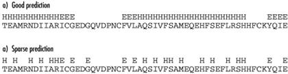
A second measure of prediction accuracy is the segment overlap score (Sov) proposed by Burkhard Rost and coworkers. The Sov metric tends to be more stringent than Q3, since it gives high scores to non-overlapping segments of a single kind of secondary structure, and penalizes sparse predictions (Figure 10-4).
Figure 10-4. Good and bad (sparse) secondary structure predictions
When comparing methods, it pays to be conservative; look at both the average scores and their standard deviations instead of the best reported score. As you can see, Q3 and Sov are fairly simple statistics. Unlike E-values reported in sequence comparison, neither is a test statistic; both measure the percent of residues predicted correctly instead of measuring the significance of prediction accuracy. And, as with genefinders, make sure you know what kind of data is used to train the prediction method.
10.5.4 Putting Predictions to Use
Originally, the goal of predicting secondary structure was to come up with the most accurate prediction possible. Many researchers took this as their goal, resulting in many gnawed fingernails and pulled-out hairs. As mentioned earlier, the hard-won lesson of secondary structure prediction is that it isn't very accurate. However, secondary structure prediction methods have practical applications in bioinformatics, particularly in detecting remote homologs. Drug companies compare secondary structure predictions to locate potential remote homologs in searches for drug targets. Patterns of predicted secondary structure can predict fold classes of proteins and select targets in structural genomics.
Secondary structure prediction tools such as PredictProtein and JPred combine the results of several approaches, including secondary structure prediction and threading methods. Using secondary structure predictions from several complementary methods (both single-sequence and homology-based approaches) can result in a better answer than using just one method. If all the methods agree on the predicted structure of a region, you can be more confident of the prediction than if it had been arrived at by only one or two programs. This is known as a voting procedure in machine learning.
As with any other prediction, secondary structure predictions are most useful if some information about the secondary structure is known. For example, if the structure of even a short segment of the protein has been determined, that data can be used as a sanity check for the prediction.
10.5.5 Predicting Transmembrane Helices
Transmembrane helix prediction is related to secondary structure prediction. It involves the recognition of regions in protein sequences that can be inserted into cell membranes. Methods for predicting transmembrane helices in protein sequences identify regions in the sequence that can fold into a helix and exist in the hydrophobic environment of the membrane. Transmembrane helix prediction grew out of research into hydrophobicity in the early 1980s, pioneered by Russell Doolittle (University of California, San Diego). Again, there are a number of transmembrane helix prediction servers available over the Web. Programs that have emerged as standards for transmembrane helix prediction include TMHMM (https://www.cbs.dtu.dk/services/TMHMM-1.0/), MEMSAT (https://insulin.brunel.ac.uk/~jones/memsat.html), and TopPred (https://www.sbc.su.se/~erikw/toppred2/).
Although structure determination for soluble proteins can be difficult, a far greater challenge is structure determination for membrane-bound proteins. Some of the most interesting biological processes involve membrane proteinsfor example, photosynthesis, vision, neuron excitation, respiration, immune response, and the passing of signals from one cell to another. Yet only a handful of membrane proteins have been crystallized. Because these proteins don't exist entirely in aqueous solution, their physicochemical properties are very different from those of soluble proteins and they require unusual conditions to crystallizeif they are amenable to crystallization at all.
As a result, many computer programs exist that detect transmembrane segments in protein sequence. These segments have distinct characteristics that make it possible to detect them with reasonable certainty. In order to span a cell membrane, an alpha helix must be about 17-25 amino acids in length. Because the interior of a cell membrane is composed of the long hydrocarbon chains of fatty acids, an alpha helix embedded in the membrane must present a relatively nonpolar surface to the membrane in order for its position to be energetically favorable.
Early transmembrane segment identification programs exploited these problems directly. By analyzing every 17-25 residue windows of an amino acid sequence and assigning a hydrophobicity score to each window, high-scoring segments can be predicted to be transmembrane helices. Recent improvements to these early methods have boosted prediction of individual transmembrane segments to an accuracy level of 90 -95%.
The topology of the protein in the membrane isn't as easy to predict. The orientation of the first helix in the membrane determines the orientation of all the remaining helices. The connections of the helices can be categorized as falling on one side or the other of the membrane, but determining which side is which, physiologically, is more complicated.
10.5.6 Threading
The basic principle of structure analysis by threadingis that an unknown amino acid sequence is fitted into (threaded through) a variety of existing 3D structures, and the fitness of the sequence to fold into that structure is evaluated. All threading methods operate on this premise, but they differ in their details.
Threading methods don't build a refined all-atom model of the protein; rather, they rapidly substitute amino acid positions in a known structure with the sidechains from the unknown sequence. Each sidechain position in a folded protein can be described in terms of its environment: to what extent the sidechain is exposed to solvent and, if it isn't exposed to solvent, what other amino acids it's in contact with. A threaded model is scored highly if hydrophobic residues are found in solvent-inaccessible environments and hydrophilic residues on the protein surface. But these high scores are possible only if buried charged and polar residues are found to have appropriate countercharges or hydrogen bonding partners, etc.
Threading is most profitably used for fold recognition, rather than for model building. For this purpose, the UCLA-DOE Structure Prediction Server (https://www.doe-mbi.ucla.edu/people/frsur/frsur.html) is by far the easiest tool to use. It allows you to submit a single sequence and try out multiple fold-recognition and evaluation methods, including the DOE lab's own Gon prediction method as well as EMBL's TOPITS method and NIH's 123D+ method. Other features, including BLAST and FASTA searches, PROSITE searches, and Bowie profiles, which evaluate the fitness of a sequence for its apparent structure, are also available.
Another threading server, the 3D-PSSM server offered by the Biomolecular Modelling Laboratory of the Imperial Cancer Research Fund, provides a fold prediction based on a profile of the unknown sequence family. 3D-PSSM incorporates multiple analysis steps into a simple interface. First the unknown protein sequence is compared to a nonredundant protein sequence database using PSI-BLAST, and a position-specific scoring matrix (PSSM) for the protein is generated. The query PSSM is compared to all the sequences in the library database; the query sequence is also compared to 1D-PSSMs (PSSMs based on standard multiple sequence alignments) and 3D-PSSMs (PSSMs based on structural alignments) of all the protein families in the library database. Secondary structure predictions based on these comparisons are shown, aligned to known secondary structures of possible structural matches for the query protein. The results from the 3D-PSSM search are presented in an easy-to-understand graphical format, but they can also be downloaded, along with carbon-alpha-only models of the unknown sequence built using each possible structural match as a template.
Most threading methods are considered experimental, and new methods are always under development. More than one method can be used to help identify any unknown sequence, and the results interpreted as a consensus of multiple experts. The main thing to remember about any structural model you build using a threading server is that it's likely to lack atomic detail, and it's also likely to be based on a slightly or grossly incorrect alignment. The threading approach is designed to assess sequences as likely candidates to fit into particular folds, not to build usable models. Putative structural alignments generated using threading servers can serve as a basis for homology modeling, but they should be carefully examined and edited prior to building an all-atom model
10.6 Predicting 3D Structure
As was stated earlier in the chapter, predicting protein structure from sequence is a difficult task, and there is no method yet that satisfies all parameters. There are, however, a number of tools that can predict 3D structure. They fall into two subgroups: homology modeling and ab-initio prediction.
10.6.1 Homology Modeling
Let's say you align a protein sequence (a 'target' sequence) against the sequence of another protein with a known structure. If the target sequence has a high level of similarity to the sequence with known structure (over the full length of the sequence), you can use that known structure as a template for the target protein with a reasonable degree of confidence.
There is a standard process that is used in homology modeling. While the programs that carry out each step may be different, the process is consistent:
Use the unknown sequence as a query to search for known protein structures.
Produce the best possible global alignment of the unknown sequence and the template sequence(s).
Build a model of the protein backbone, taking the backbone of the template structure as a model.
In regions in which there are gaps in either the target or the template, use a loop-modeling procedure to substitute
segments of appropriate length.
Add sidechains to the model backbone.
Optimize positions of sidechains.
Optimize structure with energy minimization or knowledge-based optimization.
The key to a successful homology-modeling project isn't usually the software or server used to produce the 3D model. Your skill in designing a good alignment to a template structure is far more critical. A combination of standard sequence alignment methods, profile methods, and structural alignment techniques may be employed to produce this alignment, as we discuss in the example at the end of this chapter. Once a good alignment exists, there are several programs that can use the information in that alignment to produce a structural model.
10.6.1.1 Modeller
Modeller (https://guitar.rockefeller.edu/modeller/modeller.html) is a program for homology modeling. It's available free to academics as a standalone program or as part of MSI's Quanta package (https://www.msi.com).
Modeller has no graphical interface of its own, but once you are comfortable in the command-line environment, it's not all that difficult to use. Modeller executables can be downloaded from the web site at Rockefeller University, and installation is straightforward; follow the directions in the README file available with the distribution. There are several different executables available for each operating system; you should choose based on the size of the modeling problems you will use them for. The README file contains information on the array size limits of the various executables. There are limits on total number of atoms, total number of residues, and total number of sequences in the input alignment.
As input to Modeller, you'll need two input files, an alignment file, and a Modeller script. The alignment file format is described in detail in the Modeller manpages; the Modeller script for a simple alignment consists of just a few lines written in the TOP language (Modeller's internal language). Modeller can calculate multiple models for any input. If the ENDING_ MODEL value in the example script shown is set to a number other than one, more models are generated. Usually, it's preferable to generate more than one model, evaluate each model independently, and choose the best result as your final model.
The example provided in the Modeller documentation shows the setup for an alignment with a pregenerated alignment file between one known protein and one unknown sequence:
INCLUDE # Include the predefined TOP routines
SET ALNFILE = 'alignment.ali' # alignment filename
SET KNOWNS = '5fd1' # codes of the templates
SET SEQUENCE = '1fdx' # code of the target
SET ATOMS_FILES_DIRECTORY = './:../atom_files'# directories for input atom files
SET STARTING_MODEL= 1 # index of the first model
SET ENDING_MODEL = 1 # index of the last model
# (determines how many models to calculate)
CALL ROUTINE = 'model' # do homology modeling
Modeller is run by giving the command mod scriptname. If you name your script fdx.top, the command is mod fdx.
Modeller is multifunctional and has built-in commands that will help you prepare your input:
SEQUENCE_SEARCH
Searches for similar sequences in a database of fold class representative structures
MALIGN3D
Aligns two or more structures
ALIGN
Aligns two blocks of sequences
CHECK_ ALIGNMENT
Evaluates an alignment to be used for modeling
COMPARE_SEQUENCES
Scores sequences in an alignment based on pairwise similarity
SUPERPOSE
Superimposes one model on another or on the template structure
ENERGY
Generates a report of restraint violations in a modeled structure
Each command needs to be submitted to Modeller via a script that calls that command, as shown in the previous sample script. Dozens of other Modeller commands and full details of writing scripts are described in the Modeller manual.
One caveat in automated homology modeling is that sidechain atoms may not be correctly located in the resulting model; automatic model building methods focus on building a reasonable model of the structural backbone of the protein because homology provides that information with reasonable confidence. Homology doesn't provide information about sidechain orientation, so the main task of the automatic model builder is to avoid steric conflicts and improbable conformations rather than optimize sidechain orientations. Incorrect sidechain positions may be misleading if the goal of the model building is to explore functional mechanisms.
10.6.1.2 How Modeller builds a model
Though Modeller incorporates tools for sequence alignment and even database searching, the starting point for Modeller is a multiple sequence alignment between the target sequence and the template protein sequence(s). Modeller uses the template structures to generate a set of spatial restraints, which are applied to the target sequence. The restraints limit, for example, the distance between two residues in the model that's being built, based on the distance between the two homologous residues in the template structure. Restraints can also be applied to bond angles, dihedral angles, and pairs of dihedrals. By applying enough of these spatial restraints, Modeller effectively limits the number of conformations the model can assume.
The exact form of the restraints are based on a statistical analysis of differences between pairs of homologous structures. What those statistics contribute is a quantitative description of how much various properties are likely to vary among homologous structures. The amount of allowed variation between, for instance, equivalent alpha-carbon-to-alpha-carbon distances is expressed as a PDF, or probability density function.
What the use of PDF-based restraints allows you to do, in homology modeling, is to build a structure that isn't exactly like the template structure. Instead, the structure of the model is allowed to deviate from the template but only in a way consistent with differences found between homologous proteins of known structure. For instance, if a particular dihedral angle in your template structure has a value of -60º, the PDF-based restraint you apply should allow that dihedral angle to assume a value of 60 plus or minus some value. That value is determined by what is observed in known pairs of homologous structures, and it's assigned probabilistically, according to the form of the probability density function.
Homology-based spatial restraints aren't the only restraints applied to the model. A force field controlling proper stereochemistry is also applied, so that the model structure can't violate the rules of chemistry to satisfy the spatial restraints derived from the template structures. All chemical restraints and spatial restraints applied to the model are combined in a function (called an objective function) that's optimized in the course of the model building process.
10.6.1.3 ModBase: a database of automatically generated models
The developers of Modeller have made available a queryable online database of annotated homology models. The models are prepared using an automated prediction pipeline. The first step in the pipeline is to compare each unknown protein sequence with a database of existing protein structures. Proteins that have significant sequence homology to domains of known structures are then modeled using those structures as templates. Unknown sequences are aligned to known structures using the ALIGN2D command in Modeller, and 3D structures are built using the Modeller program. The final step in the pipeline is to evaluate the models; results of the evaluation step are presented to the ModBase user as part of the search results. Since this is all standard procedure for homology-model development that's managed by a group of expert homology modelers, checking ModBase before you set off to build a homology model on your own is highly recommended.
The general procedure for building a model with Modeller is to identify homologies between the unknown sequence and proteins of known structures, build a multiple alignment of known structures for use as a template, and apply the Modeller algorithm to the unknown sequence. Models can subsequently be evaluated using standard structure-evaluation methods.
10.6.1.4 The SWISS-MODEL server
SWISS-MODEL is an automated homology modeling web server based at the Swiss Institute of Bioinformatics. SWISS-MODEL allows you to submit a sequence and get back a structure automatically. The automated procedure that's used by SWISS-MODEL mimics the standard steps in a homology modeling project:
Uses BLAST to search the protein structure database for sequences of known structure
Selects templates and looks for domains that can be modeled based on non-homologous templates
Uses a model-building program to generate a model
Uses a molecular mechanics force field to optimize the model
You must supply an unknown sequence to initiate a SWISS-MODEL run in their First Approach mode; however, you can also select the template chains that are used in the model building process. This information is entered via a simple web form. You can have the results sent to you as a plain PDB file, or as a project file that can be opened using the SWISS-PDBViewer, a companion tool for the SWISS-MODEL server you can download and install on your own machine.
Although that sounds simple, such an automatic procedure is error-prone. In a nonautomated molecular modeling project, there is plenty of room for user intervention. SWISS-MODEL actually allows you to intervene in the process using their Project Mode. In Project Mode, you can use the SWISS-PDBViewer to align your template and target sequences manually, then write out a project file, and upload it to the SWISS-MODEL server.
10.6.2 Tools for Ab-Initio Prediction
Since ab-initio structure prediction from sequence has not been done with any great degree of success so far, we can't recommend software for doing this routinely. If you are interested in the ab-initio structure-prediction problem and want to familiarize yourself with current research in the field, we suggest you start with any of these tools: the software package RAMP developed by Ram Samudrala, the I-Sites/ ROSETTA prediction server developed by David Baker and Chris Bystroff, and the ongoing work of John Moult. Recent journal articles describing these methods can serve as adequate entry points into the ab-initio protein structure prediction literature.
10.7 Putting It All Together: A Protein Modeling Project
So how do all of these tools work to produce a protein structure model from sequence? We haven't described every single point and click in this chapter, because most of the software is web-based and quite self-explanatory in that respect. However, you may still be wondering how you'd put it all together to manage a tough modeling project.
As an example, we built a model of a target sequence from CASP 4, the most recent CASP competition. We've deliberately chosen a difficult sequence to model. There are no unambiguously homologous structures in the PDB, though there are clues that can be brought together to align the target with a possible template and build a model. We make no claims that the model is correct; its purpose is to illustrate the kind of process you might go through to build a partial 3D model of a protein based on a distant similarity.
The process for building an initial homology model when you do have an obvious, strong homology to a known structure is much more straightforward: simply align the template and target along their full length, edit the alignment if necessary, write it out in a format that Modeller can read, and submit; or submit the sequence of your unknown to SWISS-MODEL in First Approach mode.
10.7.1 Finding Homologous Structures
The first step in any protein modeling project is to find a template structure (if possible) to base a homology model on.
Using the target sequence T0101 from CASP 4, identified as a '400 amino acid pectate lyase L' from a bacterium called Erwinia chrysanthemi, we searched the PDB for homologs. We started by using the PDB SearchFields form to initiate a FASTA search.
The results returned were disheartening at first glance. As the CASP target list indicated, there were no strong sequence homologies to the target to be found in the PDB. None of the matches had E-values less than 1, though there were several in the less-than-10 range. None of the matches spanned the full length of the protein, the longest matching being a 330 amino acid overlap with a chondroitinase, with an E-value of 3.9.
Each of the top scoring proteins looked different, too, as you can see in Figure 10-5. The top match was an alpha-beta barrel type structure, while the second match (the chondroitinase) was a mainly beta structure with a few decorative alpha helices, and the third match was an entirely different, multidomain all-beta structure.
Out of curiosity, we also did a simple keyword search for pectate lyase in the PDB. There were eight pectate lyase structures listed, but none, apparently, were close enough in sequence to the T0101 target to be recognized as related by sequence information alone. None of these structures was classified as pectate lyase L; they included types A, E, and C. However, we observed that each of the pectate lyase molecules in the PDB had a common structural feature: a large, quasihelical arrangement of short beta strands known as a beta solenoid, or, less picturesquely, as a single-stranded right-handed beta helix (Figure 10-6).
Figure 10-5. Pictures of top three sequence matches of a target sequence from CASP 4
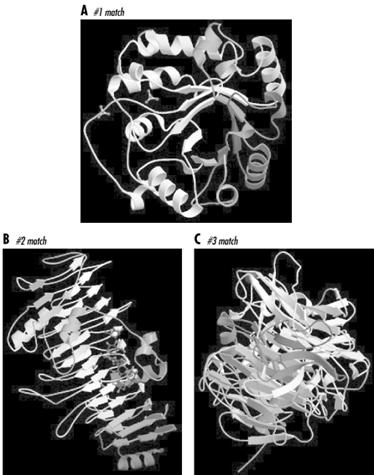
Figure 10-6. The beta-solenoid domain
10.7.2 Looking for Distant Homologies
We used CE to examine the structural neighbors of the known pectate lyases. Interestingly, one of the three proteins (1DBG, a chondroitinase from Flavobacterium heparinium) we first identified with FASTA as a sequence match for our target sequence showed up as a high-scoring structural neighbor of many of the known pectate lyases.
Although the homology between T0101 and these other pectate lyases wasn't significant, the sequence similarity between T0101 and their close structural neighbor 1DBG seemed to suggest that the structure of our target protein might be distantly related to that of the other pectate lyases (Figure 10-7). Note that the alignment in the figure shows a strongly conserved structural domainthe ladderlike structure at the right of the molecule where the chain traces coincide.
Figure 10-7. A structural alignment of known pectate lyase structures; the beta solenoid domain is visible as a ladderlike structure in the center of the molecule
However, in order to do any actual homology modeling, we need to somehow align the T0101 sequence to potential template structures. And since none of the pectate lyase sequences were similar enough to the unknown sequence to be aligned to it using standard pairwise alignment, we would need to get a little bit crafty with our alignment strategy.
10.7.3 Predicting Secondary Structure from Sequence
We applied several secondary structure prediction algorithms to the T0101 target sequence using the JPred structure prediction server. While the predictions from each method aren't exactly the same, we can see from Figure 10-8 that the consensus from JPred is clear: the T0101 sequence is predicted to form many short stretches of beta structure, exactly the pattern that is required to form the beta-solenoid domain.
Figure 10-8. Partial secondary structure predictions for T0101, from JPred
10.7.4 Using Threading Methods to Find Potential Folds
We also sent the sequence to the 3D-PSSM and 123D+ threading servers to analyze its fitness for various protein folds. The top-scoring results from the 3D-PSSM threading server, with E-values in the 95% certainty range, included the proteins 1AIR (a pectate lyase), 1DBG (the chondroitinase that was identified as a homolog of our unknown by sequence-based searching), 1IDK, and 1PCL, all pectate lyases identified by CE as structural neighbors of 1DBG. These proteins were also found in the top results from 123D+.
10.7.5 Using Profile Methods to Align Distantly Related Sequences
We now had evidence from multiple sources that suggested the structures 1AIR, 1DBG, and 1IDK would be reasonable candidates to use as templates to construct a model of the T0101 unknown sequence. However, the remaining challenge was to align the unknown sequence to the template structures. We had many different alignments to work with: the initial FASTA alignment of the unknown with 1DBG; the CE structural alignment of 1DBG and its structural neighbors 1AIR, 1DBG, and 1IDK; and the individual alignments of predicted secondary structure in the unknown to known secondary structure for each of the database hits from 3D-PSSM. Each alignment was different, of course, because they were generated by different methods. We chose to combine the information in the individual 3D-PSSM sequence-to-structure alignments of the unknown sequence with 1AIR and 1IDK into a single alignment file. We did this by aligning those two alignments to each other using Clustal's Profile Alignment mode. Finally, we wrote out the alignment to a single file in a format appropriate for Modeller and used this as input for our first approach.
10.7.6 Building a Homology Model
We created the following input for Modeller:
The input script, peclyase.top:
Homology modelling by the MODELLER TOP routine 'model'.
INCLUDE # Include the predefined TOP routines
SET ALNFILE = 'peclyase.ali' # alignment filename
SET KNOWNS = '1air','1idk' # codes of the templates
SET SEQUENCE = 't0101' # code of the target
SET ATOM_FILES_DIRECTORY = './templates' # directories for input atom files
SET STARTING_MODEL= 1 # index of the first model
SET ENDING_MODEL = 3 # index of the last model
# (determines how many models to calculate)
CALL ROUTINE = 'model' # do homology modeling
We created a sequence alignment file, peclyase.ali, in PIR format, built as described in the example and modified to indicate to Modeller whether each sequence was a template or a target.
We also placed PDB files, containing structural information for the template chains of 1AIR and 1IDK, in a templates subdirectory of our working directory. The files were named 1air.atm and 1idk.atm, as Modeller requires, and we then ran Modeller to create structural models. The models looked similar to their templates, especially in the beta solenoid domain, and evaluated reasonably well by standard methods of structure verification, including 3D/1D profiles and geometric evaluation methods. However, just like the actual CASP 4 competitors, we await the publication of the actual structure of the T0101 target for validation of our structural model.
10.8 Summary
Solving protein structure is complicated at best, but as you've seen, there are a number of software tools to make it easier. Table 1 provides a summary of the most popular structure prediction tools and techniques available to you.
Table 1. Structure Prediction Tools and Techniques
|
What you do |
Why you do it |
What you use to do it |
|
Secondary structure prediction |
As a starting point for classification and structural modeling |
JPred, Predict-Protein |
|
Threading |
To check the fitness of a protein sequence to assume a known fold; to identify distantly related structural homologs |
3D-PSSM, PhD, 123D |
|
Homology modeling |
To build a model from a sequence, based on homologies to known structures |
Modeller, SWISS-MODEL |
|
Model verification |
To check the fitness of a modeled structure for its protein sequence |
VERIFY-3D, PROCHECK, WHAT IF |
|
Ab-initio structure modeling |
To predict a 3D structure from sequence in the absence of homology |
ROSETTA, RAMP |
Chapter 11. Tools for Genomics and Proteomics
The methods we have discussed so far can be used to analyze a single sequence or structure and compare multiple sequences of single-gene length. These methods can help you understand the function of a particular gene or the mechanism of a particular protein. What you're more likely to be interested in, though, is how gene functions manifest in the observable characteristics of an organism: its phenotype. In this chapter we discuss some datatypes and tools that are beginning to be available for studying the integrated function of all the genes in a genome.
What sets genomic science apart from the traditional experimental biological sciences is the emphasis on automated data gathering and integration of large volumes of information. Experimental strategies for examining one gene or one protein are gradually being replaced by parallel strategies in which many genes are examined simultaneously. Bioinformatics is absolutely required to support these parallel strategies and make the resulting data useful to the biology community at large. While bioinformatics algorithms may be complicated, the ultimate goals of bioinformatics and genomics are straightforward. Information from multiple sources is being integrated to form a complete picture of genomic function and its expression as the pheotype of an organism, as well as to allow comparison between the genomes of different organisms. Figure 11-1 shows the sort of flowchart you might create when moving from genetic function to phenotypic expression.
Figure 11-1. A flowchart moving from genome to phenotype
From the molecular level to the cellular level and beyond, biologists have been collecting information about pieces of this picture for decades. As in the story of the blind men and the elephant, focusing on specific pieces of the biological picture has made it difficult to step back and see the functions of the genome as a whole. The process of automating and scaling up biochemical experimentation, and treating biochemical data as a public resource, is just beginning.
The Human Genome Project has not only made gigabytes of biological sequence information available; it has begun to change the entire landscape of biological research by its example. Protein structure determination has not yet been automated at the same level as sequence determination, but several pilot projects in structural genomics are underway, with the goal of creating a high-speed structure determination pipeline. The concept behind the DNA microarray experimentthousands of microscopic experiments arrayed on a chip and running in paralleldoesn't translate trivially to other types of biochemical and molecular biology experiments. Nonetheless, the trend is toward efficiency, miniaturization, and automation in all fields of biological experimentation.
A long string of genomic sequence data is inherently about as useful as a reference book with no subject headings, page numbers, or index. One of the major tasks of bioinformatics is creating software systems for information management that can effectively annotate each part of a genome sequence with information about everything from its function, to the structure of its protein product (if it has one), to the rate at which the gene is expressed at different life stages of an organism. Currently, the only way to get the functional information that is needed to fully annotate and understand the workings of the genome is traditional biochemical experimentation, one gene or protein at a time. The growing genome databases are the motivation for further parallelization and automation of biological research.
Another task of genome information management systems is to allow users to make intuitive, visual comparisons between large data sets. Many new data integration projects, from visual comparison of multiple genomes to visual integration of expression data with genome map data, are under development.
Bioinformatics methods for genome-level analysis are obviously not as advanced in their development as sequence and structure analysis methods. Sequence and structure data have been publicly available since the 1970s; a significant number of whole genomes have become available only very recently. In this chapter, we focus on some data presentation and search strategies the research community has identified as particularly useful in genomic science.
11.1 From Sequencing Genes to Sequencing Genomes
In Chapter 7, we discussed the chemistry that allows us to sequence DNA by somehow producing a ladder of sequence fragments, each differing in size by one base, which can then be separated by electrophoresis. One of the first computational challenges in the process of sequencing a gene (or a genome) is the interpretation of the pattern of fragments on a sequencing gel.
11.1.1 Analysis of Raw Sequence Data: Basecalling
The process of assigning a sequence to raw data from DNA sequencing is called basecalling. As an end user of genome sequence data, you don't have access to the raw data directly from the sequencer; you have to rely on a sequence that has been assigned to this data by some kind of processing software. While it's not likely you will actually need basecalling software, it is helpful to remember what the software does and that it can give rise to errors.
If this step doesn't produce a correct DNA sequence, any subsequent analysis of the sequence is affected. All sequences deposited in public databases are affected by basecalling errors due to ambiguities in sequencer output or to equipment malfunctions. EST and genome survey sequences have the highest error rates (1/10 -1/100 errors per base), followed by finished sequences from small laboratories (1/100 - 1/1,000 per base) and finished sequences from large genome sequencing centers (1/10,000 -1/100,000 per base).[1] Any sequence in GenBank is likely to have at least one error. Improving sequencing technology, and especially the signal detection and processing involved in DNA sequencing, is still the subject of active research.
These values were provided by Dr. Sean Eddy of Washington University.
There are two popular high-throughput protocols for DNA sequencing. As discussed earlier, DNA sequencing as it is done today relies on the ability to create a ladder of fragments of DNA at single-base resolution and separate the DNA fragments by gel electrophoresis. The popular Applied Biosystems sequencers label the fragmented DNA with four different fluorescent labels, one for each base-specific fragmentation, and run a mixture of the four samples in one gel lane. Another commonly used automated sequencer, the Pharmacia ALF instrument, runs each sample in a separate, closely spaced lane. In both cases, the gel is scanned with a laser, which excites each fluorescent band on the gel in sequence. In the four-color protocol, the fluorescence signal is elicited by a laser perpendicular to the gel, one lane at a time, and is then filtered using four colored filters to obtain differential signals from each fluorescent label. In the single-color protocol, a laser parallel to the gel excites all four lanes from a single sequencing experiment at once, and the fluorescent emissions are recorded by an array of detectors. Each of these protocols has its advantages in different types of experiments, so both are in common use. Obviously, the differences in hardware result in differences in the format of the data collected, and the use of proprietary file formats for data storage doesn't resolve this problem.
There are a variety of commercial and noncommercial tools for automated basecalling. Some of them are fully integrated with particular sequencing hardware and input datatypes. Most of them allow, and in fact require, curation by an expert user as sequence is determined.
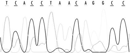
The raw result of sequencing is a record of fluorescence intensities at each position in a sequencing gel. Figure 11-2 shows detector ouput from a modern sequencing experiment. The challenge for automated basecalling software is to resolve the sequence of apparent fluorescence peaks into four-letter DNA sequence code. While this seems straightforward, there are fairly hard limits on how much sequence can be read in a single experiment. Because separation of bands on a sequencing gel isn't perfect, the quality of the separation and the shape of the bands deteriorates over the length of the gel. Peaks broaden and intermingle, and at some point in the sequencing run (usually 400 -500 bases), the peaks become impossible to resolve. Various properties of DNA result in nonuniform reactions with the sequencing gel, so that fragment mobility is slightly dependent on the identity of the last base in a fragment; overall signal intensities can depend on local sequence and on the reagents used in the experiment. Unreadable regions can occur when DNA fragments fold back upon themselves or when a sequencing primer reacts with more than one site in a DNA sequence, leading to sample heterogeneity. Because these are fairly well-understood, systematic errors, computer algorithms can be developed to compensate for them. The ultimate goal of basecalling software development is to improve the accuracy of each sequence read, as well as to extend the range of sequencing runs, by providing means to deconvolute the more ambiguous fluorescence peaks at the end of the run.
Figure 11-2. Detector output from a modern sequencing experiment
Most sequencing projects deal with the inherent errors in the sequencing process by simply sequencing each region of a genome multiple times and by sequencing both DNA strands (which results in high-quality reads of both ends of a sequence). If you read that a genome has been sequenced with 4X coverage or 10X coverage, that means that portion of the genome has been sequenced multiple times, and the results merged to produce the final sequence.
Modern sequencing technologies replace gels with microscopic capillary systems, but the core concepts of the process are the same as in gel-based sequencing: fragmentation of the DNA and separation of individual fragments by electrophoresis.
At this point, the major genome databases don't provide raw sequence data to users, and for most applications, access to raw sequence data isn't really necessary. However, it is likely that, with the constant growth of computing power, this will change in the future, and that you may want to know how to reanalyze the raw sequence data underlying the sequences available in the public databases.
One noncommercial software package for basecalling is Phred, which is available from the University of Washington Genome Center. Phred runs on either Unix or Windows NT workstations. It uses Fourier analysis to resolve fluorescence traces to predict an evenly spaced set of peak locations, then uses dynamic programming to match the actual peak locations with the predicted results. It then annotates output from basecalling with the probability that the call is an error. Phred scores represent scaled negative log probability that a base call is in error; hence, the higher the Phred score, the lower the probability that an error has been made. These values can be helpful in determining whether a region of the genome may need to be resequenced. Phred can also feed data to a sequence-assembly program called Phrap, which then uses both the sequence information and quality scores to aid in sequence assembly.
11.1.2 Sequencing an Entire Genome
Genome sequencing isn't simply a scaled-up version of a gene-sequencing run. As noted earlier, the sequence length limit of a sequencing run is something like 500 base pairs. And the length of a genome can range from tens of thousands to billions of base pairs. So in order to sequence an entire genome, the genome has to be broken into fragments, and then the sequenced fragments need to be reassembled into a continuous sequence.
There are two popular strategies for sequencing genomes: the shotgun approach and the clone contig approach. Combinations of these strategies are often used to sequence larger genomes.
11.1.2.1 The shotgun approach
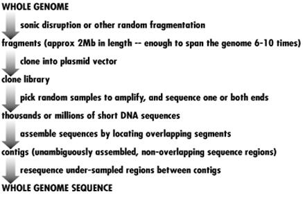
Shotgun DNA sequencing is the ultimate automated approach to DNA sequencing. In shotgun sequencing, a length of DNA, either a whole genome or a defined subset of the genome, is broken into random fragments. Fragments of manageable length (around 2,000 KB) are cloned into plasmids (together, all the clones are called a clone library). Plasmids are simple biological vectors that can incorporate any random piece of DNA and reproduce it quickly to provide sufficient material for sequencing.
If a sufficiently large amount of genomic DNA is fragmented, the set of clones spans every base pair of the genome many times. The end of each cloned DNA fragment is then sequenced, or in some cases, both ends are sequenced, which puts extra constraints on the way the sequences can be assembled. Although only 400 -500 bases at the end or ends of the fragment are sequenced, if enough clones are randomly selected from the library and sequenced, the amount of sequenced DNA still spans every base pair of the genome several times. In a shotgun sequencing experiment, enough DNA sequencing to span the entire genome 6 -10 times is usually required.
The final step in shotgun sequencing is sequence assembly, which we discuss in more detail in the next section. Assembly of all the short sequences from the shotgun sequencing experiment usually doesn't result in one single complete sequence. Rather, it results in multiple contigsunambiguously assembled lengths of sequence that don't overlap each other. In the assembly process, contigs start and end because a region of the genome is encountered from which there isn't enough information (i.e., not enough clones representing that region) to continue assembling fragments. The final steps in sequencing a complete genome by shotgun sequencing are either to find clones that can fill in these missing regions, or, if there are no clones in the original library that can fill in the gaps, to use PCR or other techniques to amplify DNA sequence that spans the gaps.
Recently, Celera Genomics has shown that shotgun DNA sequencingsequencing without a mapcan work at the whole genome level even in organisms with very large genomes. The largely completed Drosophila genome sequence is evidence of their success.
11.1.2.2 The clone contig approach
The clone contig approach relies on shotgun sequencing as well, but on a smaller scale. Instead of starting by breaking down the entire genome into random fragments, the clone contig approach starts by breaking it down into restriction fragments, which can then be cloned into artificial chromosome vectors and amplified. Restriction enzymes are enzymes that cut DNA. These enzymes are sequence-specific; that is, they recognize only one specific sequence of DNA, anywhere from 6-10 base pairs in length. By pure statistics, any base has a 1 in 4 chance of occurring randomly in a DNA sequence; an N-residue sequence has a 1 in 4N chance of occurring. Enzymes that cut at a specific 6 -10 base pair sequence of DNA end up cutting genomic DNA relatively rarely, but because DNA sequence isn't random, the restriction enzyme cuts result in a specific pattern of fragment lengths that is characteristic of a genome.
Each of the cloned restriction fragments can be sequenced and assembled by a standard shotgun approach. But assembly of the restriction fragments into a whole genome is a different sort of problem. When the genome is digested into restriction fragments, it is only partially digested. The amount of restriction enzyme applied to the DNA sample is sufficient to cut at only approximately 50% of the available restriction sites in the sample. This means that some fragments will span a particular restriction site, while other fragments will be cut at that particular site and will span other restriction sites. So the clone library that is made up of these restriction fragments will contain overlapping fragments.
Chromosome walking is the process of starting with a specific clone, then finding the next clone that overlaps it, and then the next, etc. Methods such as probe hybridization or PCR are used to help identify the restriction fragment that has been inserted into each clone, and there are a number of experimental strategies that can make building up the genome map this way less time-consuming. A genome map is a record of the location of known features in the genome, which makes it relatively simple to associate particular clone sequences with a specific location in the genome by probe hybridization or other methods.
Genomes can be mapped at various levels of detail. Geneticists are used to thinking in terms of genetic linkage maps, which roughly assign the genes that give rise to particular traits to specific loci on the chromosome. However, genetic linkage maps don't provide enough detail to support the assembly of a full genome worth of sequence, nor do they point to the actual DNA sequence that corresponds to a particular trait. What genetic linkage maps do provide, though, is a set of ordered markers, sometimes very detailed depending on the organism, which can help researchers understand genome function (and provide a framework for assembling a full genome map).
Physical maps can be created in several ways: by digesting the DNA with restriction enzymes that cut at particular sites, by developing ordered clone libraries, and recently, by fluorescence microscopy of single, restriction enzyme-cleaved DNA molecules fixed to a glass substrate. The key to each method is that, using a combination of labeled probes and known genetic markers (in restriction mapping) or by identifying overlapping regions (in library creation), the fragments of a genome can be ordered correctly into a highly specific map (see Figure 11-2).
11.1.2.3 LIMS: Tracking all those minisequences
In carrying out a sequencing project, tracking the millions of unique DNA samples that may be isolated from the genome is one of the biggest information technology challenges. It's also probably one of the least scientifically exciting, because it involves keeping track of where in the genome each sample came from, which sample goes into each container, where each container goes in what may be a huge sample storage system, and finally, which data came from which sample. The systems that manage output from high-throughput sequencing are called Laboratory Information Management Systems (LIMS), and while we will not discuss them in the context of this book, LIMS development and maintenance makes up the lion's share of bioinformatics work in industrial settings. Other high-throughput technologies, such as microarrays and cheminformatics, also require complicated LIMS support.
11.2 Sequence Assembly
Basecalling is only the first step in putting together a complete genome sequence. Once the short fragments of sequence are obtained, they must be assembled into a complete sequence that may be many thousands of times their length. The next step is sequence assembly.
Sequence assembly isn't something you're likely to be doing on your own on a large scale, unless you happen to be working for a genome project. However, even small labs may need to solve sequence-assembly problems that require some computer assistance.
DNA sequencing using a shotgun approach provides thousands or millions of minisequences, each 400 -500 fragments in length. The fragments are random and can partially or completely overlap each other. Because of these overlaps, every fragment in the set can be identified by sequence identity as adjacent to some number of other fragments. Each of those fragments overlaps yet another set of fragments, and so on. It's standard procedure for the sequences of both ends of some fragments to be known, and the sequences of only one end of other fragments to be known. Figure 11-3 illustrates the shotgun sequencing approach.
Figure 11-3. The shotgun DNA sequencing approach
Ultimately, all the fragments need to be optimally tiled together into one continuous sequence. Identifying sequence overlaps between fragments puts some constraints on how the sequences can be assembled. For some fragments, the length of the sequence and the sequences of both its ends are known, which puts even more constraints on how the sequences can be assembled. The assembly algorithm attempts to satisfy all the constraints and produce an optimal ordering of all the fragments that make up the genome.
Repetitive sequence features can complicate the assembly process. Some fragments will be uncloneable, and the sequencing process will fail in other cases, leaving gaps in the DNA sequence that must be resolved by resequencing. These gaps complicate automated assembly. If there isn't sufficient information at some point in the sequence for assembly to continue, the sequence contig that is being created comes to an end, and a new contig starts when there is sufficient sequence information for assembly to resume.
The Phrap program, available from the University of Washington Genome Center, does an effective job assembling sequence fragments, although a large amount of computer time is required. The accompanying program Consed is a Unix-based editor for Phrap sequence assembly output. TIGR Assembler is another genome assembly package that works well for small genomes, BACs, or ESTs.
11.3 Accessing Genome Informationon the Web
Partial or complete DNA sequences from hundreds of genomes are available in GenBank. Putting those sequence records together into an intelligible representation of genome structure isn't so easy. There are several efforts underway to integrate DNA sequence with higher-level maps of genomes in a user-friendly format. So far, these efforts are focused on the human genome and genomes of important plant and animal model systems. They aren't collected into one uniform resource at present, although NCBI does aim to be comprehensive in its coverage of available genome data eventually.
Looking at genome data is analogous to looking at a map of the world. You may want to look at the map from a distance, to see the overall layout of continents and countries, or you may want to find a shortcut from point A to point B. Each choice requires a different sort of map. However, the maps need to be linked, because you may want to know the general directions from San Diego to Blacksburg, VA, but may also want to know exactly how to get to a specific building on the Virginia Tech campus when you get there. The approach that web-based genome analysis tools are taking is similar to the approach taken by online map databases such as MapQuest. Place names and zip codes are analogous to gene names and GenBank IDs. You can search as specifically as you wish, or you can begin with a top view of the genome and zoom in.
The genome map resources have the same limitations as online map resources, as well. You can search MapQuest and see every street in Blacksburg, but ask MapQuest for a back-road shortcut between Cochin and Mangalore on the southwest coast of India, and it can't help you. Currently, NCBI and EMBL provide detailed maps and tools for looking at the human genome, but if your major interest is the cat genome, you're (at least this year) out of luck.
Genome resources are also limited by the capabilities of bioinformatics analysis methods. The available analysis tools at the genome sites are usually limited to sequence comparison tools and whatever single-sequence feature-detection tools are available for that genome, along with any information about the genome that can be seamlessly integrated from other databases. If you are hoping to do something with tools at a genome site you can't do with existing sequence or structure analysis tools, you will still be disappointed. What genome sites do provide is a highly automated user experience and expertly curated links between related concepts and entities. This is a valuable contribution, but there are still questions that can't be answered.
11.3.1 NCBI Genome Resources
NCBI offers access to a wide selection of web-based genome analysis tools from the Genomic Biology section of its main web site. These tools are designed for the biologist seeking answers to specific questions. Nothing beyond basic web skills and biological knowledge is required to apply these tools to a question of interest. Their interfaces are entirely point-and-click, and NCBI supplies ample documentation to help you learn how to use their tools and databases.
Here's a list of the available tools:
Genome Information
Genome project information is available from the Entrez Genomes page at NCBI. Database listings are available for the full database or for related groups of organisms such as microorganisms, archaea, bacteria, eukaryotes, and viruses. Each entry in the database is linked to a taxonomy browser entry or a home page with further links to available information about the organism. If a genome map of the organism is available, a 'See the Genome' link shows up on the organism's home page. From the home page, you can also download genome sequences and references.
Map Viewer
If a genome map is available for the organism, you can click on parts of the cartoon map that is first displayed and access several different viewing options. Depending on the genome, you can access links to overview maps, maps showing known protein-coding regions, listings of coding regions for protein and RNA, and other information. Information is generally downloadable in text format. Map Viewer distinguishes between four levels of information: the organism's home page, the graphical view of the genome, the detailed map for each chromosome (aligned to a master map from which the user can select where to zoom in), and the sequence view, which graphically displays annotations for regions of the genome sequence. Full Map Viewer functionality is available only for human and drosophila genomes at the time of this writing; however, for any complete genome, clickable genome maps and views of the annotated genome at the sequence level are available.
ORF Finder
The Open Reading Frame (ORF) Finder is a tool for locating open reading frames in a DNA sequence. ORF finders translate the sequence using standard or user-specified genetic code. In noncoding DNA, stop codons are frequently found. Only long uninterrupted stretches without stop codons are taken to be coding regions. Information from the ORF finder can provide clues about the correct reading frame for a DNA sequence and about where coding regions start and stop. For many genomes found in the Entrez Genomes database, ORF Finder is available as an integrated tool from the map view of the genome.
LocusLink
LocusLink is a curated database of genetic loci in several eukaryotic organisms that give rise to known phenotypes. LocusLink provides an alphabetical listing of traits as well as links to HomoloGene and Map Viewer.
HomoloGene
HomoloGene is a database of pairwise orthologs (homologous genes from different organisms that have diverged by speciation, as opposed to paralogs that have diverged by gene duplication) across four major eukaryotic genomes: human, mouse, rat, and zebrafish. The ortholog pairs are identified either by curation of literature reports or calculation of similarity. The HomoloGene database can be searched using gene symbols, gene names, GenBank accession numbers, and other features.
Clusters of Orthologous Groups (COG)
COG is a database of orthologous protein groups. The database was developed by comparing protein sequences across 21 complete genomes. The entries in COG represent genome functions that are conserved throughout much of evolutionary historyfunctions that were developed early and retained in all of the known complete genomes. The authors' assumption is that these ancient conserved sequences comprise the minimal core of functionality that a modern species (i.e., one that has survived into the era of genome sequencing) requires. The COG database can be searched by functional category, phylogenetic pattern, and a number of other properties.
NCBI also provides detailed genome-specific resources for several important eukaryotic genomes, including human, fruit fly, mouse, rat, and zebrafish.
11.3.2 TIGR Genome Resources
The Institute for Genome Research (TIGR, https://www.tigr.org) is one of the main producers of new genome sequence data, along with the other major human genome sequencing centers and commercial enterprises such as Celera. TIGR's main sequencing projects have been in microbial and crop genomes, and human chromosome 16. TIGR recently announced the Comprehensive Microbial Resource, a complete microbial genome resource for all of the genomes they have sequenced. At the present time, each microbial genome has its own web page from which various views of the genome are available. There are also tools within the resource that allow you to search the omniome, as TIGR designates the combined genomic information in its database. The TIGR tools aren't as visual as the NCBI genome analysis tools. Selection of regions to examine requires you to enter specific information into a form rather than just pointing and clicking on a genome map. However, the TIGR resources are a useful supplement to the NCBI tools, providing a different view on the same genetic information.
TIGR maintains many genome-specific databases focused on expressed sequence tags (ESTs) rather than complete genomic data. ESTs are partial sequences from either end of a cDNA clone. Despite their incompleteness, ESTs are useful for experimental molecular biologists. Since cDNA libraries are prepared by producing the DNA complement to cellular mRNA (messenger RNA), a cDNA library gives clues as to what genes are actually expressed in a particular cell or tissue. Therefore, a sequence match with an EST can be an initial step in helping to identify the function of a new gene. TIGR's EST databases can be searched by sequence, EST identifier, cDNA library name, tissue, or gene product name, using a simple forms-based web interface.
11.3.3 EnsEMBL
EnsEMBL is a collaborative project of EMBL, EBI, and the Sanger Centre (https://www.sanger.ac.uk) to automatically track sequenced fragments of the human genome and assemble them into longer stretches. Automated analysis methods, such as genefinding and feature-finding tools and sequence-comparison tools, are then applied to the assembled sequence and made available to users through a web interface.
In June 2000, the Human Genome consortium announced the completion of the first map of the human genome. It's important to stress that such maps, and indeed much of the genomic information now available, are only drafts of a final picture that may take years to assemble. To remain useful, the draft maps must be constantly updated to stay in sync with the constantly updated sequence databases. The EnsEMBL project expects to apply its automated data analysis pipeline to many different genomes, beginning with human and mouse.
There are three ways to search EnsEMBL: a BLAST search of a query sequence against the database; a search using a known gene, transcript, or map marker ID; or a chromosome map browser that allows you to pick a chromosome and zoom in to ever-more specific regions. All these tools are relatively self-explanatory and available from the EnsEMBL web site. In order to use them, however, you should know something of what you are looking for or on which chromosome to look.
11.3.4 Other Sequencing Centers
TIGR isn't the only genome center to provide software and online tools for analyzing genomic data. Genome sequencing programs generally incorporate a bioinformatics component and attract researchers with interests in developing bioinformatics methods; their web sites are good points of entry to the bioinformatics world. The University of Washington Genome Center is known for the development of sequence assembly toolsits Phred and Phrap software are widely used. Other genome centers include, but aren't limited to, the Sanger Centre, the DOE Joint Genome Institute, Washington University in St. Louis, and many corporate centers.
A complete list of genome sequencing projects in progress and active genome centers can be found online in the Genomes OnLine Database (GOLD), a public site maintained by Integrated Genomics, Inc. (https://wit.integratedgenomics.com/GOLD/).
11.3.5 Organism-Specific Resources
The Arabidopsis Information Resource (TAIR) is an excellent example of an organism-specific genome resource, this one focusing on the widely used plant model system Arabidopsis thaliana. In addition to the standard features offered at EnsEMBL and NCBI, such as clickable and zoomable chromosome maps and sequence analysis tools, TAIR offers a variety of expert-curated links to other information for users of the resource. TAIR is limited in its scope to Arabidopsis, but it is a much deeper resource than the general public databases. Similar resources are available for many organisms, from maize to zebrafish. Listings of online genome resources can be located at several sites, such as GOLD, NCBI, and EMBL.
11.4 Annotating and Analyzing Whole Genome Sequences
Genome data presents completely new issues in data storage and analysis:
Genome sequences are extremely large.
Users need to access genome data both as a whole and as meaningful pieces.
The majority of the sequence in a genome doesn't correspond to known functionality.
Annotation of the genome with functional information can be accomplished by several means: comparison with existing information for the organism in the sequence databases, comparison with published information in the primary literature, computational methods such as ORF detection and genefinding, or propagation of information from one genome to another by evolutionary inference based on sequence comparison. Due to the sheer amount of data available, automatic annotation is desirable, but it must be automatic without propagating errors. The use of computational methods is fallible; sequence similarity searches can result in hits that aren't biologically meaningful, and genefinders often have difficulty detecting the exact start and end of a gene. Sometimes experimental information is incorrect or is recorded incorrectly in the database. Using this information to annotate genomes leaves a residue of error in the database, which can then be propagated further by use of comparative methods.
11.4.1 Genome Annotation
Genome annotation is a difficult business. This is in part because there are a huge number of different pieces of information attached to every gene in a genome. Not every piece of information is interesting to every user, and not every piece of this information can (or should) be crammed in a single file of information about the gene. Genome annotation relies on relational databases to integrate genome sequence information with other data.[2]
The term relational database should give you a clue that the function of the database is to maintain relationships or connections among entries. We discuss this in more detail in Chapter 13.
The primary sources of information about what genes do are laboratory experiments. It may take many experiments to figure out what a gene does. Ideally, all that diverse experimental data should somehow be associated with the gene annotation. What this means in practice is hyperlinking of content between multiple databasessequence, structure, and functional genomics fully linked together in a queryable system. This strategy is beginning to be implemented in most of the major public databases, although the goal of 'one world database' (in the user's perception) has not yet been reached and perhaps never will.
11.4.1.1 MAGPIE
MAGPIE is an environment for annotation of genomes based on sequence similarity. It can maintain status information for a genome project and make information about the genome available on the Web, as well as provide an interface for automated sequence similarity-based and manual annotation. Even if you're not maintaining a genome database for public use, a look at the features of MAGPIE may help clarify some of the information technology issues in genome annotation. The Sulfolobus solfataricus P2 Genome Project and many other smaller genome projects have implemented MAGPIE; the S. solfataricus project provides information on its web site about the role MAGPIE plays in the genome annotation process.
11.4.2 Genome Comparison
Pairwise or multiple comparison of genomes is an idea that will be useful for many studies, ranging from basic questions of evolutionary biology to very specific clinical questions, such as the identification of genetic polymorphisms, which give rise to disease states or significant variations in phenotype.
Why compare whole genomes rather than just comparing genes one at a time? As the Human Genome Project reaches completion, researchers are just beginning to explore in detail how genome structure affects genome function. Is junk DNA really junk? Are there structural features in DNA that control expression? Are there promoters and regulatory regions we haven't yet figured out? Genome comparison can help answer such questions by pointing to regions of similarity within uncharacterized or even supposedly redundant DNA. Genome comparison will also aid in genomic annotation. Prototype genome comparisons have helped to justify the sequencing of additional genomes; the comparison of mouse and human genomes is one such example. Genome comparison is useful both at the map level and directly at the sequence level.
11.4.2.1 PipMaker
PipMaker is a tool that compares two DNA sequences of up to 2 MB each (longer sequences will be handled by the new Version 2.0, to be released soon) and produces a percent identity plot as output. This is useful in identifying large-scale patterns of similarity in longer sequences, although obviously not entire larger genomes. The process of using PipMaker is relatively simple. Starting with two FASTA-format sequence files, you first generate a set of instructions for masking sequence repeats (generated using the RepeatMasker server). This reduces the number of uninformative hits in the sequence comparison. The resulting information, plus a simple file containing a numerical list of known gene positions, is submitted to the PipMaker web server at Penn State University and the results are emailed to you. A detailed PipMaker tutorial is available at the web site (https://bio.cse.psu.edu/pipmaker/). PipMaker relies on BLASTZ to align sequences. BLASTZ is an experimental version of BLAST designed for extremely long sequences and developed at NCBI.
11.4.2.2 MUMmer
Another program for pairwise genome comparison is TIGR's MUMmer. MUMmer was designed to meet the needs of the sequencing projects at TIGR and is optimized for comparing microbial genome sequences that are assumed to be relatively similar. Its first application was a detailed comparison of genomes of two strains of M. tuberculosis. MUMmer can compare sequences millions of base pairs in length and produce colorful visualizations of regions of similarity. MUMmer is based on a computer algorithm called a suffix tree, which essentially makes it easy for the system to rapidly handle a large number of pairwise comparisons. The dynamic programming algorithm used in standard BLAST comparison doesn't scale well with sequence length. For genome-length sequences, dynamic programming methods are unacceptably slow. MUMmer is an example of a novel method developed to get around the problems involved in using standard pairwise sequence comparison to compare full genome sequences. MUMmer is designed for Unix systems and is freely available for use in nonprofit institutions. A new public web interface to MUMmer has recently become available on the TIGR web site.
11.5 Functional Genomics: New Data Analysis Challenges
The advent of high-speed sequencing methods has changed the way we study the DNA sequences that code for proteins. Once, finding these bits of DNA in the genome of an organism was the goal, without much concern for the context. It is now becoming possible to view the whole DNA sequence of a chromosome as a single entity and to examine how the parts of it work together to produce the complexity of the organism as a whole.
The functions of the genome break down loosely into a few obvious categories: metabolism, regulation, signaling, and construction. Metabolic pathways convert chemical energy derived from environmental sources (i.e., food) into useful work in the cell. Regulatory pathways are biochemical mechanisms that control what genomic DNA does: when it is expressed and when it isn't. Genomic regulation involves not only expressed genes but structural and sequence signals in the DNA where regulatory proteins may bind. Signaling pathways control, among other things, the movement of chemicals from one compartment in a cell to another. Teasing out the complex networks of interactions that make up these pathways is the work of biochemists and molecular biologists. Many regulatory systems for the control of DNA transcription have been studied. Mapping these metabolic, regulatory, and signaling systems to the genome sequence is the goal of the field of functional genomics.
11.5.1 Sequence-Based Approaches for Analyzing Gene Expression
In addition to genome sequence, GenBank contains many other kinds of DNA sequence. Expressed sequence tag (EST) data for an organism can be an extremely useful starting point for discovery-oriented exploration of gene expression. To understand why this is, you need to recall what ESTs represent. ESTs are partial sequences of cDNA clones; cDNA clones are DNA strands built using cellular mRNA as templates.[3] In the cell, mRNA is RNA with a missionto be converted into protein, and soon. mRNA levels respond to changes in the cell or its environment; mRNA levels are tissue-dependent, and they change during the life cycle of the organism as well. Quantitation of mRNA or cDNA provides a pretty good measure of what a genome is doing under particular conditions.
The term transcriptome has been used to describe the collection of sequenced transcripts from a given organism.
The sequence of a cDNA molecule built off an mRNA template should be the same as the sequence of the DNA that originally served as a template for building the mRNA. Sequencing a short stretch of bases from a cDNA sequence provides enough information to localize the source of an mRNA in a genome sequence.
NCBI offers a database called dbEST that provides access to several thousand libraries of ESTs. Quite a large number of these are human EST libraries, but there are libraries from dozens of other organisms as well. NCBI's UniGene database provides fully searchable access to specific EST libraries from human, mouse, rat, and zebrafish. EST data within UniGene has been combined with sequences of well-characterized genes and clustered, using an automated clustering procedure, to identify groups of related sequences. The Library Browser can locate libraries of interest within UniGene.
Another NCBI resource for sequence-based expression analysis is SAGEmap. Serial Analysis of Gene Expression (SAGE) is an experimental technique in which the transcription products of many genes are rapidly quantitated by sequencing short 'tags' of DNA at a specific position (usually a restriction site) in the sequence. SAGEmap is a specialized online resource for the SAGE user community that identifies potential SAGE tags in human DNA sequence and maps them to the genome.
11.5.2 DNA Microarrays: Emerging Technologiesin Functional Genomics
Recently, new technology has made it possible for researchers to rapidly explore expression patterns of entire genomes worth of DNA. A microarray (or gene chip) is a small glass slidelike a microscope slideabout a centimeter on a side. The surface of the slide is covered with 20,000 or more precisely placed spots each containing a different DNA oligomer (short polynucleotide chain). cDNA can also be affixed to the slide to function as probes. Other media, such as thin membranes, can be used in place of slides. The key to the experiment is that each piece of DNA is immobilizedattached at one end to the slide's surface. Any reaction that results in a change in microarray signal can be precisely assigned to a specific DNA sequence.
Microarray experiments capitalize on an important property of DNA. One strand of DNA (or RNA) can hybridize with a complementary strand of DNA. If the complementarity of the two strands is perfect, the bond between the two strands is difficult to break. Each oligomer in a DNA microarray can serve as a probe to detect a unique, complementary DNA or RNA molecule. These oligomers can be bound by fluorescently labeled DNA, allowing the chip to be scanned using a confocal scanner or CCD camera. The presence or absence of a complementary sequence in the DNA sample being run over the chip determines whether the position on the array 'lights up' or not. Thus, the presence or absence of an average of 20,000 sequences can be experimentally demonstrated with one gene chip.
Microarrays are conceptually no different from traditional hybridization experiments such as Southern Blots (probing DNA samples separated on a filter with labeled probe sequences) or Northern Blots (probing RNA samples separated on a filter). In traditional blotting, the protein sample is immobilized; in microarray experiments, the probe is immobilized, and the amount of information that can be collected in one experiment is vastly larger. Figure 11-4 shows just a portion of a microarray scan from Arabidopsis (Image courtesy of the Arabidopsis Functional Genomics Consortium (AFGC) and the Stanford Microarray Database, https://genome-www.stanford.edu/microarray). Other advantages are that microarray experiments rely on fluorescent probes rather than the radioactive probes used in blotting techniques, and gene chips can be manufactured robotically rather than laboriously generated by hand.
Figure 11-4. A microarray scan
Microarray technology is now routinely used for DNA sequencing experiments; for instance, in testing for the presence of polymorphisms. Another recent development is the use of microarrays for gene expression analysis. When a gene is expressed, an mRNA transcript is produced. If DNA oligomers complementary to the genes of interest are placed on the microarray, mRNA or cDNA copies can be hybridized to the chip, providing a rapid assay as to whether or not those genes are being expressed. Experiments like these have been performed in yeast to test differences in whole-genome expression patterns in response to changes in ambient sugar concentration. Microarray experiments can provide information about the behavior of every one of an organism's genes in response to environmental changes.
11.5.3 Bioinformatics Challenges in Microarray Design and Analysis
So why do microarrays merit a section in a book on bioinformatics? Bioinformatics plays multiple roles in microarray experiments. In fact, it is difficult to conceive of microarrays as useful without the involvement of computers and databases. From the design of chips for specific purposes, to the quantitation of signals, to the extraction of groups of genes with linked expression profiles, microarray analysis is a process that is difficult, if not impossible, to do by eye or with a pencil and a notebook.
The most popular laboratory equipment for microarray experiments, at the time of this writing, is the Affymetrix machine; however, it's been followed closely by home-built configurations. If you're working with a commercial arrayer, integrated software will probably make it relatively easy for you to analyze data. However, home-built microarray setups put out data sets of varying sizes. Arrayers may not spot quite as uniformly as commercial machines. Standardization is difficult. And running a home-built setup means you have to find software that supports all the steps of the array experiment and has the features you need for data analysis.
One of the main challenges in conducting microarray experiments with noncommercial equipment is that there are a limited number of available tools for linking expression data with associated sequences and annotations. Constructing such a database interface can be a real burden for a novice. Proprietary software, based on proprietary chip formats, is often quite well supported by a database backend specific to the chip, but it isn't always generalizable, or not easily so, to a variety of image formats and data-set sizes. In the public domain, several projects are underway to improve this situation for academic researchers, including NCGR's GeneX and EMBL-EBI's ArrayExpress. The National Human Genome Research Institute (NHGRI) is currently offering a demonstration version of an array data management system called ArrayDB (https://genome.nhgri.nih.gov/arraydb/) that includes both analysis tools and relational database support.[4] ArrayDB will also allow a community of users to add records to a central database.
It's in alpha release at the time of this writing.
The Pat Brown group at Stanford has a comprehensive listing of microarray resources on their web site, including instructions for building your own arrayer (for about 10% of the cost of a commercial setup) and the ArrayMaker software that controls the printing of arrays. This site is an excellent resource for microarray beginners.
11.5.3.1 Planning array experiments
A key element in microarray experiments is chip design. This is the aspect that's often forgotten by users of commercial devices and commercial chips, because one benefit of those systems is that chip design has been done for you, by an expert, before you ever think about doing an experiment. Chip design is a process that can take months.
Even the largest chip can't fit all the proteins in a eukaryotic genome; there may be hundreds of thousands of different targets. The chip designer has to select subsets of the genome that are likely to be informative when assayed together. EST data sets can be helpful in designing microarray primers; while they are quantitatively uninformative, ESTs do indicate which subsets of genes are likely to be active under particular conditions and hence are informative for a specific microarray experiment.
In order for microarray results to be clear and unambiguous, each DNA probe in the array must be sufficiently unique that only one specific target gene can hybridize with it. Otherwise, the amount of signal detected at each spot will be quantitatively incorrect.
What this means, in practice, is lots of sequence analysis: finding possible genes of interest, and selecting and synthesizing appropriate probes. Once the probes are selected, their sequence, plus available background information for each spot in the array, must be recorded in a database so that information is accessible when results are analyzed. Finally, the database must be robust enough to take into account changing annotations and information in the public sequence databases, so that incorrect interpretations of results can be avoided.
Some resources for probe and primer design are available on the Web. A 'good' oligonucleotideone that is useful as a probe or primer for microarrays, PCR, and other hybridization experiments shouldn't hybridize with itself to form dimers or hairpins. It should hybridize uniquely with the target sequence you are interested in. For PCR applications, primers must have an optimal melting temperature and stability. An excellent web resource for designing PCR primers is the Primer3 web site at the Whitehead Institute; CODEHOP is another primer/probe design application based on sequence motifs found in the Blocks database.
11.5.3.2 Analyzing scanned microarray images with CrazyQuant
Once the array experiment is complete, you'll find yourself in possession of a lot of very large TIFF files containing scanned images of your arrays. If you're not using an integrated analysis package, where do you go from there?
The standard for public-domain microarray analysis tools are the packages developed at Stanford. One package, ScanAlyze, available for Windows, is the image analysis tool in this group. ScanAlyze is well regarded and widely used, especially in academia and features semiautomatic grid definition and multichannel pixel analysis. It supports TIFF files as well as the Stanford SCN format. It's by far the most sophisticated of the image-analysis programs discussed here.
A relatively straightforward public-domain program for array-image analysis is CrazyQuant, a Java application available from the Hood Laboratory at the University of Washington. CrazyQuant is menu-driven and can load TIFF, JPG, or GIF format microarray images. CrazyQuant assumes a 2D matrix of regularly spaced spots, and to begin the analysis process, you need to define a 2D grid that pinpoints the spot locations. The program then computes relative intensities at each spot and stores them as integer values. CrazyQuant can quantitate both one- and two-color (differential) array data. CrazyQuant is extremely simple to install on a Linux workstation. Download the archive, move it to its own directory, unzip it, and run the program by entering java CrazyQuant. A sample GIF image is included in the archive so that you can see how it works.
TIGR also offers a Windows application for microarray image analysis called SpotFinder. SpotFinder can process the TIFF-format files produced by most microarray scanners and produce output that is compatible with both TIGR's ArrayViewer and other microarray analysis software.
11.5.3.3 Visualizing high-dimensional data
Microarray results can be difficult to visualize. Array experiments generally have at least four dimensions (x-location, y-location, fluorescence intensity, and time). Straightforward plotting of array images isn't very informative. Tools that help extract features from higher-dimensional data sets and display these features in a sensible image format are needed.
TIGR offers a Java application called ArrayViewer. Currently, ArrayViewer's functions are focused on detecting differentially expressed genes and displaying differential expression results in a graphical format. ArrayViewer's parameters can be adjusted to incorporate data from arrays of any size, and it can be configured to allow straightforward access to underlying gene sequence data and annotation. Several normalization options are offered. Features for analysis of time series data and other more complicated data sets aren't yet implemented, but ArrayViewer does meet most basic array visualization needs.
Some general visualization and data-mining packages such as Xgobi, which we discuss in Chapter 14, can also be used to examine array data.
11.5.3.4 Clustering expression profiles
At the time of this writing, the most popular strategy for analysis of microarray data is the clustering of expression profiles. An expression profile can be visualized as a plot that describes the change in expression at one spot on a microarray grid over the course of the experiment. The course of the experiment changes with the context, anything from changes in the concentration of nutrients in the medium in which cells are being grown prior to having their DNA hybridized to the array, to cell cycle stages.
In this context, what is clustered is essentially the shape of the plot. Different clustering methods, such as hierarchical clustering or SOMs (self-organizing maps) may work better in different situations, but the general aim of each of these methods is the same.[5] If two genes change expression levels in the same way in response to a change in conditions, it can be assumed that those genes are related. They may share something as simple as a promoter, or more likely, they are controlled by the same complex regulatory pathway. Automated clustering of expression profiles looks for similar symptoms (similarly shaped expression profiles) but doesn't necessarily point to causes for those changes. That's the job of the scientist analyzing the results, at least for now.
We discuss clustering approaches in a little more detail in Chapter 14.
The programs Cluster and TreeView, also from Stanford, are Windows-platform tools for clustering expression profiles. Various algorithms for clustering are implemented, including SOMs and hierarchical clustering. XCluster, which implements most of the features of Cluster, is available for Unix platforms. All these programs require a specific file format (detailed in the manual, which is available online).
11.5.3.5 A note on commercial software for expression analysis
Several commercial software packages, with tools for visualizing complex microarray data sets, are available. Many of these are specific to particular hardware or array configurations. Others, such as SpotFire and Silicon Genetics' GeneSpring, are more universal. These software packages are often rather expensive to license; however, at this stage of the development of microarray technology, their relative ease of use may make them worthwhile.
11.6 Proteomics
Proteomics refers to techniques that simultaneously study the entire protein complement of a cell. While protein purification and separation methods are constantly improving, and the time-to-completion of protein structures determined by NMR and x-ray crystallography is decreasing, there is as yet no single way to rapidly crystallize the entire protein complement of an organism and determine every structure. Techniques in biochemical characterization, on the other hand, are getting better and faster. The technological advance in biochemistry that most requires informatics support is the immobilized-gradient 2D-PAGE process and the subsequent characterization of separated protein products by mass spectrometry. Microarraying robots have begun to be used to create protein arrays, which can be used in protein interaction assays, drug discovery, and other applications. However, protein microarrays are still far from a routine approach.
11.6.1 Experimental Approaches in Proteomics
Knowing when and at what levels genes are being expressed is only the first step in understanding how the genome determines phenotype. While mRNA levels are correlated with protein concentration in the cell, proteins are subject to post-translational modifications that can't be detected with a hybridization experiment. Experimental tools for determining protein concentration and activity in the cell are the crucial next step in the process.
Another high-throughput technology that is emerging as a tool in functional genomics is 2D gel electrophoresis. Gels have long been used in molecular biology to separate mixtures of components. Depending on the conditions of the experiment and the type of gel used, different components will migrate through a gel matrix at different rates. (This same principle makes DNA sequencing possible).
Two-dimensional gel electrophoresis can be used to separate protein mixtures containing thousands of components. The first dimension of the experiment is separation of the components of a solution along a pH gradient (isoelectric focusing). The second dimension is separation of the components orthogonally by molecular weight. Separation in these two dimensions can resolve even a complicated mixture of components. Figure 11-5 shows a 2D-PAGE reference map from Arabidopsis thaliana. The 2D-PAGE experiment separates proteins from a mixed sample so that individual proteins can be identified. Each spot on the map represents a different protein. (Image Swiss Institute of Bioinformatics, Geneva, Switzerland.)
While 2D gel electrophoresis is a useful and interesting technology in itself, the technology did not really come into its own until the development of standardized immobilized-gradient gels. These gels allow very precise protein separations, resulting in standardized high density data arrays. They can therefore be subjected to automated image analysis and quantitation and used for accurate comparative studies. The other advance that has put 2D gel technology at the forefront of modern molecular biology methods is the capacity to chemically analyze each spot on the gel using mass spectrometry. This allows the measurable biochemical phenomenonthe amount of protein found in a particular spot on the gelto be directly connected to the sequence of the protein found at that spot.
Figure 11-5. A 2D-PAGE reference map from Arabidopsis thaliana
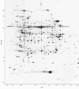
11.6.2 Informatics Challenges in 2D-PAGE Analysis
The analysis pathway for 2D-PAGE gel images is essentially quite similar to that for microarrays. The first step is an image analysis, in which the positions of spots on the gel are identified and the boundaries between different spots are resolved. Molecular weight and isoelectric point (PI) for each protein in the gel can be estimated according to position.
Next, the spots are identified, and sequence information is used to make the connection between a particular spot and its gene sequence. In microarray experiments, this step is planned in advance, as the primers or cDNA fragments are laid down in the original chip design. In proteome analysis, the immobilized proteins can either be sequenced in situ or spots of protein can be physically removed from the gel, eluted, and analyzed using mass spectrometry methods such as electrospray ionization-mass spectrometry (ESI-MS) or matrix-assisted laser desorption ionization mass spectrometry (MALDI).
The essence of mass spectrometry methods is that they can determine the masses of components in a mixture, starting from a very small sample. Proteins, fragmented by various chemically specific digestion methods, have characteristic fingerprints (patterns of peptide masses) that can identify specific proteins and match them with a gene sequence.
Peptide fingerprints are sufficient to identify proteins only in cases in which the sequence of a protein is already known and can be found in a database. When full sequence information isn't available, a second mass spectrometry step can obtain partial sequence information from each individual peptide that makes up the peptide fingerprint. The initial peptide fingerprinting process separates the protein into peptides and characterizes them by mass. Within the mass spectrometer, each peptide can then be further broken down into ionized fragments. The goal of the peptide fragmentation step is to produce a ladder of fragments each differing in length by one amino acid. Because each type of amino acid has a different molecular weight, the sequence of each peptide can be deduced from the resulting mass spectrum.
Finally, staining, radiolabeling, fluorescence, or other methods are used to quantitate each protein spot on the gel. Both in the microarray experiment and the 2D-PAGE experiment, quantitation is a fairly difficult step. In this step, computer algorithms can help analyze the amount of signal at each spot and deconvolute complex patterns of spots.
11.6.3 Tools for Proteomics Analysis
Several public-domain programs for proteomics analysis are available on the Web. Most of these can be accessed through the excellent proteomics resource at Expert Protein Analysis System (ExPASy, https://www.expasy.ch/tools/), the excellent resource maintained by the Swiss Institute of Bioinformatics. ExPASy is linked with SWISS-PROT, an expert-curated database of protein sequence information, and TrEMBL, the computer-generated counterpart to SWISS-PROT. Most of its tools are web-based and tied into these and other protein databases. The Swiss Institute of Bioinformatics also maintains SWISS-2DPAGE, a database of reference gel maps that are fully searchable and integrated with other protein information. SWISS-2DPAGE, like other biological databases, is growing rapidly; however deposition of 2D-PAGE results into databases isn't, at this time, required for publication, so the database isn't comprehensive.
The Melanie3 software package, a Windows-based package for 2D-PAGE image analysis, was developed at ExPASy, although it has since been commercialized. A Melanie viewer, which allows users who don't own Melanie3 to view Melanie3 data sets generated by colleagues, is freely distributed by ExPASy.
Here are some other ExPASy proteomics tools:
AACompIdent
Allows you to identify proteins by their amino acid composition
AACompSim
Compares a protein's amino acid composition with other proteins in SWISS-PROT
MultiDent
A multifunction tool that uses PI, molecular weight, mass fingerprints, and other data to help identify proteins
PeptIdent
Compares experimentally determined mass fingerprints with theoretically calculated mass fingerprints for all proteins in SWISS-PROT
FindMod
Predicts specific post-translational modifications to proteins based on mass differences between experimental and computed fingerprints
GlycoMod
Predicts oligosaccharide modifications from mass differences
PeptideMass
Computes a theoretical mass fingerprint for a SWISS-PROT or TrEMBL entry, or for a user-entered protein sequence
These tools are entirely forms-based and very approachable for the novice user. In addition, ExPASy provides links to many externally developed tools and web servers. It is an excellent starting resource for anyone interested in proteomics.
The PROWL database is a relatively new web resource for proteomics. PROWL tools can be used to search a protein database with peptide fingerprint or partial sequence information. The PROWL group also provides a suite of software for mass spectrometry data analysis.
11.6.4 Generalizing the Array Approach
Integration of microarray and 2D-PAGE methodswhich provide information about gene transcription and translation, respectivelywith genome sequence data is the best way currently available to form a picture of whole-genome function. However, these methods are still fairly new. Although the technology is moving forward by leaps and bounds, their results aren't yet fully standardized, and consensus software tools and analysis methods for these types of data are still emerging.
Array and 2D-PAGE experiments have elements in common, including the ability to separate and quantitate components in a mixture and fix particular components consistently to positions in a grid, and the ability to measure changes in signal at each position over time. Approaches for analyzing array-formatted biochemical data are likely to be similar on some level, whether the experiments involve DNA-DNA, DNA-mRNA, or even protein-protein interactions. Array strategies have recently been used to conduct a genome-wide survey of protein-protein interactions in yeast, and other applications of the strategy are, no doubt, in the works. Array methods and other parallel methods promise to continue to revolutionize biology. However, the biology community is still in the process of developing standards for reporting and archiving array data, and it is unlikely that a consensus will be reached before this book goes to press.
11.7 Biochemical Pathway Databases
Gene and protein expression are only two steps in the translation of genetic code to phenotype. Once genes are expressed and translated into proteins, their products participate in complicated biochemical interactions called pathways, as shown in Figure 11-6 (the image in the figure is Kyoto Encyclopedia of Genes and Genomes). It is highly unlikely that one enzyme-catalyzed chemical reaction will produce a needed product from a material readily available to the organism. Instead, a complicated series of steps is usually required. Each pathway may supply chemical precursors to many other pathways, meaning that each protein has relationships not only to the preceding and following biochemical steps in a single pathway, but possibly to steps in several pathways. The complicated branchings of metabolic pathways are far more difficult to represent and search than the linear sequences of genes and genomes.
Figure 11-6. A complex metabolic pathway
11.7.1 Illustration of a Complex Metabolic Pathway
Several web-based services offer access to metabolic pathway information. These resources are primarily databases of information linked by search tools; at the time of this writing metabolic simulation tools, such as those we describe in the next section, have not been fully integrated with databases of known metabolic pathway information into a central web-based resource.
11.7.2 EC Nomenclature
Enzymes (proteins that catalyze metabolic reactions) can be described using a standard code called the EC code. The EC nomenclature is a hierarchical naming scheme that divides enzymes into several major classes. The first class number refers to the chemistry of the enzyme: oxidoreductase, lyase, hydrolase, transferase, isomerase, or ligase. The second class number indicates what class of substrate the enzyme acts on. The third class number, which can be omitted, indicates other chemical participants in the reaction. Finally, the fourth number narrows the search to the specific enzyme. Thus, EC number 1.1.1.1 refers to alcohol dehydrogenase, which is a (1) oxidoreductase acting on the (1) CH-OH group of donors with (1) NADH as acceptor. If you are interested in using most metabolic pathway resources, it's helpful to become familiar with EC nomenclature. The EC code and hierarchy of functional definitions can be found online at the IUBMB Biochemical Nomenclature Committee web site.
11.7.3 WIT and KEGG
The best known metabolic pathway resources on the Web are What is There (WIT, https://wit.mcs.anl.gov/WIT2/) and the Kyoto Encyclopedia of Genes and Genomes (KEGG, https://www.genome.ad.jp/kegg/). WIT is a metabolic pathway reconstruction resource; that is, the curators of WIT are attempting to reconstruct complete metabolic pathway models for organisms whose genomes have been completely sequenced. WIT currently contains metabolic models for 39 organisms. The WIT models include far more than just metabolism and bioenergetics; they range from transcription and translation pathways to transmembrane transport to signal transduction.
WIT can be searched and queried in a number of ways. You can browse the database beginning at the very top level, a functional overview of the WIT contents, which is found under the heading General Overview on the main page. Each heading in the metabolic outline is a clickable link that takes you to increasingly specific levels of detail about that subset of metabolism. The View Models menu takes you directly to organism-specific metabolic models.
The General Search function allows you to search all of WIT, or subsets of organisms. This type of search is based on keywords, using Unix-style regular expressions to find matches. There is also a similarity search function that allows you to search all the open reading frames (ORFs) of a selected organism for sequence pattern matches, using either BLAST or FASTA. Pathway queries require you to specify the names of metabolites and/or specific EC enzyme codes. Enzyme queries allow you to specify an enzyme name or EC code, along with location information such as tissue specificity, cellular compartment specificity, or organelle specificity. In all except the regular-expression searches, the keywords are drawn from standardized metabolic vocabularies. WIT searches require some prior knowledge of these vocabularies when you submit the query. WIT was primarily designed as a tool to aid its developers in producing metabolic reconstructions, and documentation of the vocabularies used may not always be sufficient for the novice user. WIT is relatively text-heavy, although at the highest level of detail, metabolic pathway diagrams can be displayed.
Another web-based metabolic reconstruction resource is KEGG, which provides its metabolic overviews as map illustrations, rather than text-only, and can be easier to use for the visually-oriented user. KEGG also provides listings of EC numbers and their corresponding enzymes broken down by level, and many helpful links to sites describing enzyme and ligand nomenclature in detail. The LIGAND database, associated with KEGG, is a useful resource for identifying small molecules involved in biochemical pathways. Like WIT, KEGG is searchable by sequence homology, keyword, and chemical entity; you can also input the LIGAND ID codes of two small molecules and find all of the possible metabolic pathways connecting them.
11.7.4 PathDB
PathDB is another type of metabolic pathway database. While it contains roughly the same information as KEGG and WITidentities of compounds and metabolic proteins, and information about the steps that connect these entitiesit handles information in a far more flexible way than the other metabolic databases. Instead of limiting searches to arbitrary metabolic pathways and describing pathways with preconceived images, PathDB allows you to find any set of connected reactions that link point A to point B, or compound A to compound B.
PathDB contains, in addition to the usual search tools, a pathway visualization interface that allows you to inspect any selected pathway and display different representations of the pathway. The PathDB developers plan to incorporate metabolic simulation into the user interface as well, although those features aren't available at the time of this writing.
The PathDB browser is a platform-independent tool you can use on any machine with a Java Runtime Environment ( JRE) Version 1.1.4 or later installed. Both Sun and IBM supply a JRE for Linux systems. Once the JRE is installed, you can run the PathDB installer, making sure that the installer uses the correct version of the JRE (for this to work, you may need to add the JRE binary directory to your path). Let the installer create a link to PathDB in your home directory. To run the program, enter PathDB. You may be prompted to specify the correct Java virtual machine or exit; use the same Java pathway you did when you installed the software.
To sample how PathDB works, submit a simple query that will assure you get results the first time (such as 'All Catalysts with EC Number like 1.1.1.1,' which brings up a list of alcohol dehydrogenases). You can also follow the tutorials available from the PathDB web site.
11.8 Modeling Kinetics and Physiology
A new 'omics' buzzword that has begun to crop up in the literature rather recently is 'metabolomics.' Researchers have begun to recognize the need to exhaustively track the availability and concentration of small moleculeseverything from electrolytes to metabolic intermediates to enzyme cofactorsin biological systems. Small molecules are extremely important in biochemistry, playing roles in everything from signal transduction to bioenergetics to regulation. The populations of small molecules that interact with proteins in the cell will continue to be a key topic of research as biologists attempt to assemble the big picture of cellular function and physiology.
Mathematical modeling of biochemical kinetics and physiology is a complicated topic that is largely beyond the scope of this book. Mathematical models are generally system-specific, and to develop them requires a detailed understanding of a biological system and a facility with differential equations. However, a few groups have begun to develop context-independent software for developing biochemical and physiological models. Some of the best known of these are Gepasi, a system for biochemical modeling; XPP, a more general package for dynamical simulation; and the Virtual Cell portal.
The essential principle behind biochemical and physiological modeling is that changes in biochemical systems can be modeled in terms of chemical concentrations and associated rate equations. Each 'pool' of biochemical reagent in a system has an associated rate of formation and rate of breakdown, and the model is capable of predicting how the system will behave over time under various starting conditions. A model of metabolism may consist of dozens of reagents, each being formed and consumed by multiple reactions. Models that accurately simulate the behavior of a complex biochemical pathway aren't trivially developed, but once created, they can predict the effect of perturbations to the system and help researchers develop new hypotheses.
If you're coming from a biological sciences background, you are probably familiar with the Michaelis-Menten model for describing enzyme kinetics. Biochemical modeling extends this relatively simple mathematical model of a single enzyme-catalyzed reaction to encompass multiple reactions that may feed back upon each other in complex ways. Physiological models also involve multiple compartments with barriers through which only some components can diffuse or be transported. However, the underlying principles are similar, no matter how complex the model.
11.8.1 Modeling Kinetics with Gepasi
Gepasi (https://www.gepasi.org/) is a user-friendly biochemical kinetics simulator for Windows/NT that can model systems of up to 45 metabolites and 45 rate equations. The Gepasi interface includes interactive tools for creating a new metabolic model: entering chemical reactions, adding metabolites that may be effectors or inhibitors of the reactions, defining reaction kinetics, setting metabolite concentrations, and other key steps in model development. You can apply Gepasi's predefined reaction types to your model or define your own reaction types. Gepasi automatically checks on mass conservation relations that need to be accounted for in the simulation. Gepasi has numerous options for running simulations over various time courses and testing the results of changing variable values over a user-defined range. Gepasi can also optimize metabolic models used in metabolic engineering and fit experimental data to metabolic models.
At the time of this writing, versions of Gepasi for platforms other than Windows/NT are in development.
11.8.2 XPP
XPP (https://www.math.pitt.edu/~bard/xpp/xpp.html) is a dynamical systems simulation tool that is available for both Windows/NT and Linux. While it lacks some of the user-friendly features of Gepasi, it has been used effectively to model biochemical processes ranging from biochemical reactions to cell cycles and circadian rhythms. XPP compiles easily on any Linux system with a simple make command; just download the archive, move it into a directory of its own, extract it, then compile the program. Documentation, as well as example files for various simulations, are included with the XPP distribution.
11.8.3 Using the Virtual Cell Portal
The Virtual Cell portal at the National Resource for Cell Analysis and Modeling (NRCAM, https://www.nrcam.uchc.edu) is the first web-based resource for modeling of cellular processes. It allows you to model cells with an arbitrary number of compartments and complex physiology. A tutorial available at the Virtual Cell site walks the first-time user through the process of developing a physiology model for a cell, choosing a cell geometry, and setting up and running a simulation. The cell physiology model includes not only a compartmentation scheme for the cell, which can be created using simple drawing tools, but the addition of specific types of ionic species and membrane transporters to the cell model.
The Virtual Cell is a Java applet, which is fully supported for Macintosh and Windows users. In order to use the Virtual Cell portal on a Linux workstation, you need to download the Java plug-in for Netscape (available from https://www.blackdown.org) and install it in your ~/.netscape directory. Once the plug-in is installed, you can follow the 'MacIntosh Users Run the Virtual Cell' link on the main page, even if you're running the VCell Applet on a Linux workstation, and you can try out most features of the portal. At the time of this writing, Unix users aren't explicitly supported at the Virtual Cell portal, and while correct functionality seems to be available when the Blackdown Java applet is used, it might be wise for serious users of the VCell tools to compare results for some test cases on a Linux workstation and another machine.
11.9 Summary
We've compiled a quick-reference table of genomics and proteomics tools and techniques (Table 11-1).
Table 11-1. Genomics and Proteomics Tools and Techniques
|
What you do |
Why you do it |
What you use to do it |
|
Online genome resources |
To find information about the location and function of particular genes in a genome |
NCBI tools, TIGR tools, EnsEMBL, and genome-specific databases |
|
Basecalling |
To convert fluorescence intensities from the sequencing experiment into four-letter sequence code |
Phred |
|
Genome mapping and assembly |
To organize the sequences of short fragments of raw DNA sequence data into a coherent whole |
Phrap, Staden package |
|
Genome annotation |
To connect functional information about the genome to specific sequence locations |
MAGPIE |
|
Genome comparison |
To identify components of genome structure that differentiate one organism from another |
PipMaker, MUMmer |
|
Microarray image analysis |
To identify and quantitate spots in raw microarray data |
CrazyQuant, SpotFinder, ArrayViewer |
|
Clustering analysis of microarray data |
To identify genes that appear to be expressed as linked groups |
Cluster, TreeView |
|
2D-PAGE analysis |
To analyze, visualize, and quantitate 2D-PAGE images |
Melanie3, Melanie Viewer |
|
Proteomics analysis |
To analyze mass spectrometry results and identify proteins |
ExPASy tools, ProteinProspector, PROWL |
|
Metabolic pathway tools |
To search metabolic pathways and discover functional relationships; to reconstruct metabolic pathways |
PATH-DB, WIT, KEGG |
|
Metabolic andcellular simulation |
To model metabolic and cellular processes based on known properties and inference |
Gepasi, XPP, Virtual Cell |
As we've seen in previous chapters, a vast assortment of software tools exists for bioinformatics. Even though it's likely that someone has already written what you need, you will still encounter many situations in which the best solution is to do it yourself. In bioinformatics, that often means writing programs that sift through mountains of data to extract just the information you require. Perl, the Practical Extraction and Reporting Language, is ideally suited to this task.
12.1 Why Perl?
There are a lot of programming languages out there. In our survey of bioinformatics software, we have already seen programs written in Java, C, and FORTRAN. So, why use Perl? The answer is efficiency.[1] Biological data is stored in enormous databases and text files. Sorting through and analyzing this data by hand (and it can be done) would take far too long, so the smart scientist writes computer tools to automate the process. Perl, with its highly developed capacity to detect patterns in data, and especially strings of text, is the most obvious choice. The next obvious choice would probably be Python. Python, the less well known of the two, is a fully object-oriented scripting language introduced by Guido van Rossum in 1988. Python has some outstanding contributed code, including a mature library for numerical methods, tools for building graphical user interfaces quickly and easily, and even a library of functions for structural biology. At the end of the day, however, it's the wealth of existing Perl code for bioinformatics, the smooth integration of that code onto Unix-based systems, cross-platform portability, and an incredibly enthusiastic user community that makes Perl our favorite scripting language for bioinformatics applications.
[1] Efficiency from the programmer's point of view, that is. It takes far less programming time to extract data with Perl than with C or with Java.
Perl has a flexible syntax, or grammar, so if you are familiar with programming in other languages such as C or BASIC, it is easy to write Perl code in a C-like or BASIC-like dialect. Perl also takes care of much of the dirty work involved in programming, such as memory allocation, so you can concentrate on solving the problem at hand. It's often the case that programming problems requiring many lines of code in C or Java may be solved in just a few lines of Perl.
Many excellent books have been written about learning and using Perl, so this single chapter obviously can't cover everything you will ever need to know about the language. Perl has a mountain of features, and it's unrealistic to assume you can master it without a serious commitment to learning the art of computer programming. Our aim in this chapter isn't to teach you how to program in Perl, but rather to show you how Perl can help you solve certain problems in bioinformatics. We will take you through some examples that are most immediately useful in real bioinformatics research, such as reading datafiles, searching for character strings, performing back-of-the-envelope calculations, and reporting findings to the user. And we'll explain how our sample programs work. The rest is up to you. The ability to program in any languagebut especially in Perl, Python, or Javais an important skill for any bioinformatician to have. We strongly suggest you take a programming class or obtain one of the books on our list of recommended reading and start from the beginning. You won't regret it.
12.1.1 Where Do I Get Perl?
Perl is available for a variety of operating systems, including Windows and Mac OS, as well as Linux and other flavors of Unix. It's distributed under an open source license, which means that it's essentially free. To obtain Perl from the Web, go to https://www.perl.com/pub/language/info/software.html and follow the instructions for downloading and installing it on your system.
12.2 Perl Basics
Once you've installed Perl, or confirmed with your system administrator that it's already installed on your system, you're ready to begin writing your first program. Writing and executing a Perl program can be broken into several steps: writing the program (or script) and saving it in a file, running the program, and reading the output.
12.2.1 Hello World
A Perl program is a text file that contains instructions written in the Perl language. The classic first program in Perl (and many other languages) is called 'Hello, World!' It's written like this:
#!/usr/bin/perl -w
# Say hello
print 'Hello, World!n';
'Hello, World!' is a short program, but it's still complete. The first line is called the shebang line and tells the computer that this is a Perl program. All Perl programs running on Unix begin with this line.[2] It's a special kind of comment to the Unix shell that tells it where to find Perl, and also instructs it to look for optional arguments. In our version of 'Hello World!' we've included the optional argument -w at the end of the line. This argument tells Perl to give extra warning messages if you do something potentially dangerous in your program. It's a good idea to always develop your programs under -w.
[2] Strictly speaking, the shebang line isn't necessary on Windows or Macintosh; neither of those systems has a usr/bin/perl. It's good programming form to always include the line, however, since it's the best place to indicate your optional arguments in Perl. On other platforms, you can run the program by invoking the Perl interpreter explicitly, as in perl hello.pl.
The second line starts with a # sign. The # tells Perl that the line of text that follows is a comment, not part of the executable code. Comments are how humans tell each other what each part of the program is intended to do. Make a habit of including comments in your code. That way you and other people can add to your code, debug it successfully, and even more importantly, remember what it was supposed to do in the first place.
The third line calls the print function with a single argument that consists of a text string. At the end of the text string, there is a n, which tells the computer to move to a new line after executing the print statement. The print statement ends with a semicolon, as do most statements in Perl.
To try this little program yourself, you can open a text editor such as vi, Emacs, or pico, and type the lines in. When you've finished entering the program, name the file hello.pl and save it in your directory of choice. While you're learning, you might consider creating a new directory (using the mkdir command, which we covered in Chapter 4) called Perl in your home directory. That way you'll always know where to look for your Perl programs.
Now make the file executable using the command:
% chmod +x hello.pl
(If you need a refresher on chmod, this would be a good time to review the section on changing file permissions in Chapter 4.) To run the program, type:
% hello.pl
Because of the shebang line in our program, this command invokes the Perl interpreter, which reads the rest of the file and then translates your Perl source code into machine code the computer can execute. In this case you'll notice that Hello, World! appears on your computer screen, and then the cursor advances to a new line. You've now written and run your first Perl program!
12.2.2 A Bioinformatics Example
One of the strengths of Perland the reason that bioinformaticians love itis that with a few lines of code, you can automate a tedious task such as searching for a nucleotide string contained in a block of sequence data. To do this, you need a slightly more complex Perl program that might look like this:
#!/usr/bin/perl -w
# Look for nucleotide string in sequence data
my $target = 'ACCCTG';
my $search_string =
'CCACACCACACCCACACACCCACACACCACACCACACACCACACCACACCCACACACACA'.
'CATCCTAACACTACCCTAACACAGCCCTAATCTAACCCTGGCCAACCTGTCTCTCAACTT'.
'ACCCTCCATTACCCTGCCTCCACTCGTTACCCTGTCCCATTCAACCATACCACTCCGAAC';
my @matches;
# Try to find a match in letters 1-6 of $search_string, then look at letters 2-7,
# and so on. Record the starting offset of each match.
foreach my $i (0..length $search_string)
# Make @matches into a comma-separated list for printing
print 'My matches occurred at the following offsets: @matches.n';
print 'donen';
This program is also short and simple, but it's still quite powerful. It searches for the target string 'ACCCTG' in a sequence of data and keeps track of the starting location of each match. The program demonstrates variables and loops, which are two basic programming constructs you need to understand to make sense of what is going on.
12.2.3 Variables
A variable is a name that is associated with a data value, such as a string or a number. It is common to say that a variable stores or contains a value. Variables allow you to store and manipulate data in your programs; they are called variables because the values they represent can change throughout the life of a program.
Our sequence matching program declares four variables: $target , $search_string, @matches, and $i. The $ and @ characters indicate the kind of variable each one is. Perl has three kinds of variables built into the language: scalars, arrays, and hashes.
Unlike other programming languages, Perl doesn't require formal declaration of variables; they simply exist upon their first use whether you explicitly declare them or not. You may declare your variables, if you'd like, by using either my or our in front of the variable name. When you declare a variable, you give it a name. A variable name must follow two main rules: it must start with a letter or an underscore (the $ and @ characters aren't considered part of the name), and it must consist of letters, digits, and underscores. The best names are ones that clearly, concisely, and accurately describe the variable's role in the program. For example, it is easier to guess the role of a variable if it is named $target or $sequence, than if it were called $icxl.
12.2.3.1 Scalars
A scalar variable contains a single piece of data that is either a number or a string. The $ character indicates that a variable is scalar. The first two variables declared in our program are scalar variables:
my $target = 'ACCCTG';
my $search_string =
'CCACACCACACCCACACACCCACACACCACACCACACACCACACCACACCCACACACACA'.
'CATCCTAACACTACCCTAACACAGCCCTAATCTAACCCTGGCCAACCTGTCTCTCAACTT'.
'ACCCTCCATTACCCTGCCTCCACTCGTTACCCTGTCCCATTCAACCATACCACTCCGAAC';
In this case, 'ACCCTG' is the target string we are seeking, and 'CCACACCACACCCACAC' is the sequence data in which we're hoping to find it.
In a scalar variable, a number can be either an integer (0, 1, 2, 3, etc.) or a real number (a number that contains a fractional portion, such as 5.6). A string is a chunk of text that's surrounded by quotes. For example:
'I am a string.'
'I, too, am a string'
One of Perl's special features is that it has a number of built-in facilities for manipulating strings, which comes in handy when working with the flat text files common to bioinformatics. We cover flat text files and their more structured relatives, relational databases, in detail in Chapter 13.
12.2.3.2 Arrays
An array is an ordered list of data. In our sequence matching program, @matches is an array variable used to store the starting locations of all the matches. Each element stored in an array can be accessed by its position in the list, which is represented as a number. In Perl, array variables are given an @ prefix. For example, the following statement declares an array of numbers:
@a = ( 1, '4', 9 );
This statement declares an array of strings:
@names = ('T. Herman', 'N. Aeschylus', 'H. Ulysses', 'Standish');
And this statement declares an array with both:
@mix = ('Caesar Augustus', 'Tiberius', 18, 'Caligula', 'Claudius');
Note the syntax in the declarations: each element in the array is separated from its neighbors by a comma, each of the strings is quoted, and (unlike American English) the comma appears outside of the quotes.
Because an array is an ordered set of information, you can retrieve each element in an array according to its number. The individual elements in an array are written as $this_array[i], where i is the index of the array element being addressed. Note that i can be either a bare number (such as 21), or a numeric scalar variable (such as $n) that contains a bare number. Here is a Perl statement that uses the print operator to display the second number in @a and the third name in @names on the screen:
print 'second number: $a[1]n third name: $names[2]n';
You may be wondering why the element numbers here are one less than what you might think they should be. The reason is that positions in Perl arrays are numbered starting from zero. That is, the first element in an array is numbered 0, the second element is numbered 1, and so on. That's why, in the previous example, the second element in @a is addressed as $a[1]. This is an important detail to remember; mistakes in addressing arrays due to missing that crucial zero element are easy to make.
12.2.3.3 Hashes
A hash is also known as an associative array because it associates a name (or key, as it's called in Perl) with each piece of data (or value) stored in it. A real-world example of a hash is a telephone book, in which you look up a person's name in order to find her telephone number. Our sequence matching program doesn't use any hashes, but they can be quite handy in bioinformatics programs, as you'll see in a later example. Perl uses the % prefix to indicate hash variables (e.g., %sequences). There are a number of ways to declare a hash and its contents as a list of key/value pairs. Here is the syntax for one declaration style:
%hash = (
key1 => 'value1',
key2 => 'value2',
last_key => 'last_value' );
A value can then be retrieved from this hash using the corresponding key, as follows:
$value = $hash;
For example, you can declare a hash that relates each three-letter amino acid code to its one-letter symbol:
my %three_to_one = (
ALA => A, CYS => C, ASP => D, GLU => E,
PHE => F, GLY => G, HIS => H, ILE => I,
LYS => K, LEU => L, MET => M, ASN => N,
PRO => P, GLN => Q, ARG => R, SER => S,
THR => T, VAL => V, TRP => W, TYR => Y
);
The hash entry with the one-letter code for arginine can then be displayed using the following statement:
print 'The one-letter code for ARG is $three_to_onen';
Because there are many popular sequence databases, another place where hashes can be immediately useful is in keeping track of which sequence ID in one database corresponds to a sequence ID in the next. In the following example, we define a hash in which each of the keys is a GenBank identifier (GI) number of a particular enzyme, and each value is the corresponding SWISS-PROT identifier of the same enzyme. Using this hash, a program can take the more cryptic GI number and automatically find the associated SWISS-PROT ID:
#!/usr/bin/perl -w
# define the hash relating GI numbers to SWISSPROT IDs
%sods = (
g134606 => 'SODC_DROME',
g134611 => 'SODC_HUMAN',
g464769 => 'SODC_CAEEL',
g1711426 => 'SODC_ECOLI' );
# retrieve a value from %sods
$genbank_id = 'g134611';
$swissprot_id = $sods;
print '$genbank_id is the same as $swissprot_idn';
If you save the previous script to a file, make the file executable, and run it, you should see:
g134611 is the same as SODC_HUMAN
In the first part of this script, you are declaring the hash relating GenBank IDs to SWISS-PROT IDs. In the second part, you access the information stored in that hash. The first step is to assign one of the GenBank IDs to the variable $genbank_id. Then you can retrieve the SWISS-PROT ID that %sods has associated with the string in $genbank_id, and store the SWISS-PROT ID in the variable $swissprot_id. Finally, print the values of the two scalar variables. This example is obviously rather contrived, but it should give you an idea of how useful hashes can be in bioinformatics programs.
12.2.4 Loops
Now that we've talked about scalar, array, and hash variables in Perl, let's return to our sequence matching program and talk about the other main programming construct it employs. A loop is a programming device that repeatedly executes a specific set of commands until a particular condition is reached. Our program uses a foreach loop to iterate through the search string:
foreach my $i (0..length $search_string)
The first time through this loop, Perl starts at 0 and looks at the first six-letter combination in the search string, compares it to the target string, and, if there is a match, records it in @matches. The second cycle of the loop looks at letters 2-7, the third looks at letters 3 -8, and so on. Perl stops executing this sequence when it reaches the end of the search string. At this point, the loop is done, and the program moves on to the next section, where it prints the results. Don't worry if you don't understand all the code in the loop; all that's important right now is that you have a general understanding of what the code is doing.
12.2.5 Subroutines
Although we don't use them in any of our example programs, the use of subroutines in programs is worth mentioning. All modern programming languages provide a way to bundle up a set of statements into a subroutine so that they can be invoked concisely and repeatedly. In Perl, you can create a subroutine with the sub declaration:
sub greet
Once this greet subroutine has been declared, you can invoke it as follows:
greet('world'); # Prints 'Hello, world!'
greet('Per'); # Prints 'Hello, Per!'
Here, 'world' and 'Per' are argumentsvalues passed into the subroutine, where they are then stored in $name. Our greet subroutine just prints a single line and then returns. Usually, subroutines do something a bit more complicated, possibly returning a value:
$length = calculate_length($sequence);
This sets $length to whatever the calculate_length( ) subroutine returns when provided with the single argument $sequence. When a subroutine is used for its return value, it's often called a function.
12.3 Pattern Matching and Regular Expressions
A major feature of Perl is its pattern matching, and particularly its use of regular expressions. A regular expression (or regex in the Perl vernacular) is a pattern that can be matched against a string of data. We first encountered regular expressions in our discussion of the Unix command grep, back in Chapter 5. grep, as you may recall, searches for occurrences of patterns in files. When you tell grep to search for a pattern, you describe what you're looking for in terms of a regular expression. As you know, much of bioinformatics is about searching for patterns in data.
Let's look at a Perl example. Say you have a string, such as a DNA sequence, and you want to make sure that there are no illegal characters in it. You can use a regular expression to test for illegal characters as follows:
#!/usr/bin/perl
# check for non-DNA characters
my $string = 'CCACACCACACCCACACaCCCaCaCATCACACCACACACCACACTACACCCA*CACACACA';
if( $string =~ m/([^ATCG])/i)
This program contains the regular expression [^ATCG]. Translated into English, the regular expression says 'look for characters in $string that don't match A, T, C, or G.' (The i at the end of the statement tells Perl to match case insensitively; that is, to pay no attention to case. Perl's default is to treat A differently from a.) If Perl encounters something other than the declared pattern, the program prints out the offending character. The output of this program is:
Warning! Found * in the string
If instead you want to search for a particular combination of letters, like 'CAT', you can change the regular expression to read CAT:
#!/usr/bin/perl
# check for CATs
my $string =
'CCACACCACACCCACACaCCCaCaCATCACACCACACACCACACTACACCCA*CACACACA';
if( $string =~ m/CAT/i )
The output of this modified program is:
Meow.
12.4 Parsing BLAST Output Using Perl
Now that you know enough about how Perl is written to understand these simple programs, let's apply it to one of the most common problems in bioinformatics: parsing BLAST output. As you already know, the result of a BLAST search is often a multimegabyte file full of raw data. The results of several searches can quickly become overwhelming. But by writing a fairly simple program in Perl, you can automate the process of looking for a single string or multiple strings in your data.
Consider the following block of data:
gb|AC005288.1|AC005288 Homo sapiens chromosome 17, clone hC 268 2e-68
gb|AC008812.7|AC008812 Homo sapiens chromosome 19 clone CTD 264 3e-67
gb|AC009123.6|AC009123 Homo sapiens chromosome 16 clone RP1 262 1e-66
emb|AL137073.13|AL137073 Human DNA sequence from clone RP11 260 5e-66
gb|AC020904.6|AC020904 Homo sapiens chromosome 19 clone CTB 248 2e-62
>gb|AC007421.12|AC007421 Homo sapiens chromosome 17, clone hRPC.1030_O_14,
complete sequence
Query: 3407 accgtcataaagtcaaacaattgtaacttgaaccatcttttaactcaggtactgtgtata 3466
||||||||||||||||||||||||||||||||||||||||||||||||||||||||||||
Sbjct: 1366 accgtcataaagtcaaacaattgtaacttgaaccatcttttaactcaggtactgtgtata 1425
Query: 3467 tacttacttctccccctcctctgttgctgcagatccgtgggcgtgagcgcttcgagatgt 3526
||||||||||||||||||||||||||||||||||||||||||||||||||||||||||||
Sbjct: 1426 tacttacttctccccctcctctgttgctgcagatccgtgggcgtgagcgcttcgagatgt 1485
Query: 3527 tccgagagctgaatgaggccttggaactcaaggatgcccaggctgggaaggagccagggg 3586
||||||||||||||||||||||||||||||||||||||||||||||||||||||||||||
Sbjct: 1486 tccgagagctgaatgaggccttggaactcaaggatgcccaggctgggaaggagccagggg 1545
Query: 3587 ggagcagggctcactccaggtgagtgacctcagccccttcctggccctactcccctgcct 3646
||||||||||||||||||||||||||||||||||||||||||||||||||||||||||||
Sbjct: 1546 ggagcagggctcactccaggtgagtgacctcagccccttcctggccctactcccctgcct 1605
Query: 3647 tcctaggttggaaagccataggattccattctcatcctgccttcatggtcaaaggcagct 3706
This is only a small portion of what you might find in a report from a BLAST search. (This is actual data from a BLAST report. The entire file, blast.dat, is too large to reproduce here.) The first six lines of this sample contain information about the BLAST search, as well as other 'noise' that's of no importance to the search. The next 13 lines, and the ones that follow it in the actual report, contain the data to analyze. You want the Perl program to look at both the 'Query' and 'Sbjct' lines in this BLAST report and find the number of occurrences of the following substrings:
'gtccca'
'gcaatg'
'cagct'
'tcggga'
Missing data (represented by dashes in the nucleotide sequence strings)
At the same time, you want the program to ignore irrelevant material such as information about the search and other noise. The program should then generate a report file called report.txt that describes the findings for these strings.
In this program you need to create two very long scalar variables to represent each sequence for searching. Let's call them $query_src, and $sbjct_src. In any BLAST output, you'll notice that sometimes the 'Sbjct' and 'Query' lines aren't contiguous; that is, there are gaps in the data. From a programming perspective, the fact that the gaps exist isn't important; you simply want to read the nucleotides into your scalars consecutively. Here is a sample portion of BLAST data:
Query: 1165 gagcccaggagttcaagaccagcctgggtaacatgatgaaacctcgtctctac 1217
|||| |||||||| ||||||||||||| |||| | ||||||| ||||||||
Sbjct: 11895 gagctcaggagtttgagaccagcctggggaacacggtgaaaccctgtctctac 11843
Query: 1170 caggagttcaagaccagcctg 1190
|||||||||||||||||||||
Sbjct: 69962 caggagttcaagaccagcctg 69942
Query: 1106 tggtggctcacacctgcaatcccagcact 1134
||||||||||| |||| ||||||||||||
Sbjct: 77363 tggtggctcacgcctgtaatcccagcact 77335
In spite of the fact that the line numbers aren't contiguous, the sequence for 'Query' starts with 'gagccca' and still ends with 'agcact', and will be 103 (53 + 21 + 29) characters long. As you'll see shortly, the program is designed to ignore the gaps (and the line numbers) and input the data properly. Frequent BLAST users may also notice that in a full BLAST report, each sequence is grouped by E-values. We are ignoring that (usually) important fact in the program.
The Perl program used to search for the five substrings can be broken down into three parts:
Inputting the data and preparing it for analysis
Searching the data and looking for the patterns
Compiling the results and storing them in report.txt
Let's go through the program step by step. Here are the first few lines:
#!/usr/bin/perl
# Search through a large datafile, looking for particular sequences
use strict;
my $REPORT_FILE = 'report.txt';
my $blast_file = $ARGV[0] || 'blast.dat';
unless ( -e $blast_file )
This code makes sure that the data is in good order. Since you'll be reading large amounts of data into the variables, tell Perl to tighten up its rules with the line use strict;. This forces you to be more explicit about how you want Perl to do things. use strict is particularly useful when developing large programs or programs you want to modify and reuse. Go on to declare some variables, and in the last few lines, tell Perl to make sure that data actually exists in the input file blast.dat.
In the next block of code, the program reads the sequences into variables:
# First, slurp all the Query sequences into one scalar. Same for the
# Sbjct sequences.
my ($query_src, $sbjct_src);
# Open the blast datafile and end program (die) if we can't find it
open (IN, $blast_file) or die '$0: ERROR: $blast_file: $!';
# Go through the blast file line by line, concatenating all the Query and
# Sbjct sequences.
while (my $line = <IN>) elsif ($line =~ /^Sbjct/)
# We've now read the blast file, so we can close it.
close IN;
Once you've read the data into @words, you then instruct the program to take only the data from column two of @words (which is filled only with nucleotide sequence data) and store it in the variables $query_src and $sbjct_src. The program then closes the file and moves to a new line. You now have just the data you want, stored in a form you can use.
The next part of the program performs the analysis:
# Now, look for these given sequences
my @patterns = ('gtccca', 'gcaatg', 'cagct', 'tcggga', '-');
# and when we find them, store them in these hashes
my (%query_counts, %sbjct_counts);
# Search and store the sequences
foreach my $pattern (@patterns) ++;
}
while ( $sbjct_src =~ /$pattern/g ) ++;
}
The program sets up a loop that runs five times; once for each search string or pattern. Within each iteration of the outer foreach loop, the program runs inner while loops that advance counters each time they find a pattern match. The results are stored in separate hashes called %query_counts and %sbjct_counts.
Here is the last section of the program, which produces the output:
# Create an empty report file
open (OUT, '>$REPORT_FILE') or die '$0: ERROR: Can't write $REPORT_FILE';
# Print the header of the report file, including
# the current date and time
print OUT 'Sequence Reportn',
'Run by O'Reilly on ', scalar localtime, 'n',
'nNOTE: In the following reports, a dash (-) representsn',
' missing data in the chromosomal sequencenn',
'Total length of 'Query' sequence: ',
length $query_src, ' charactersn', 'Results for 'Query':n';
# Print the Query matches
foreach my $key ( sort @patterns ) n';
print OUT 'nTotal length of 'Sbjct' sequence: ',
length $sbjct_src, ' charactersn', 'Results for 'Sbjct':n';
# Print the Sbjct matches
foreach my $key ( sort @patterns ) n';
close OUT;
__END__
This code compiles and formats the results and dumps them into a file called report.txt. If you open report.text you see:
Sequence Report
Run by O'Reilly on Tue Jan 9 15:52:48 2001
NOTE: In the following reports, a dash (-) represents
missing data in the chromosomal sequence
Total length of 'Query' sequence: 1115 characters
Results for 'Query':
'-' seen 7
'cagct' seen 11
'gcaatg' seen 1
'gtccca' seen 6
'tcggga' seen 1
Total length of 'Sbjct' sequence: 5845 characters
Results for 'Sbjct':
'-' seen 12
'cagct' seen 2
'gcaatg' seen 6
'gtccca' seen 1
'tcggga' seen 6
In this example the results were sent to a file. You can just as easily ask Perl to generate an HTML-coded file you can view with your web browser. Or you can make the process interactive and use Perl to create a CGI script that generates a web form to analyze the data and give you back your results.
We've only scratched the surface in terms of what this sort of program can do. You can easily modify it to look for more general patterns in the data or more specific ones. For example, you might search for `tcggga' and `gcaatg', but only count them if they are connected by `cagct'. You also might search only for breaks in the data. And after all the searches are complete, you might use Perl to automatically store all the results in a database.
If you're feeling a little confused by all this, don't panic. We aren't expecting you to understand all the code we've shown you. As we said at the beginning of the chapter, the purpose of the code isn't to teach you to program in Perl, but to show you how Perl works, and also to show you that programming isn't really all that difficult. If you have what it takes to design an experiment, then you have what it takes to program in Perl or any other language.
12.5 Applying Perl to Bioinformatics
The good news is the more you practice programming, the more you learn. And the more you learn, the more you can do. Programming in Perl is all about analyzing data and building tools. As we've said before, biological data is proliferating at an astounding rate. The only chance biologists have of keeping up with the job of analyzing it is by developing libraries of reusable software tools. In Perl, there are a huge number of reusable functions available for use in your programs. Rather than being wrapped in a complete program, a group of related functions are packaged as a module. In your programs, you can use various modules to access the functions they support. There are Perl modules for other scientific disciplines, as well as games, graphics programming, video, artificial intelligence, statistics, and music. And they're all free.
To distinguish them from other Perl files, modules have a .pm suffix. To use functions from a module (say, CGI.pm) in your Perl programs, include the following line after the shebang line:
use CGI;
The primary source of all modules is the Comprehensive Perl Archive Network, or CPAN. CPAN (https://www.cpan.org) is a collection of sites located around the world, each of which mirrors the contents of the main CPAN site in Finland. To find the CPAN site nearest you, check the Perl web site (https://www.perl.com).
Because there are so many modules available, before you sit down to write a new function, it is worth your time to check the CPAN archive to see if anyone has already written it for you. In this section, we briefly describe some Perl modules that are particularly useful for solving common problems in bioinformatics. This list is by no means comprehensive; you should keep an eye on CPAN for current developments.
12.5.1 Bioperl
The Bioperl Project (along with its siblings, Biopython, BioJava, and Bioxml) is dedicated to the creation of an open source library of modules for bioinformatics research. The general idea is that common items in bioinformatics (such as sequences and sequence alignments) are represented as objects in Bioperl. Thus, if you use Bioperl, instead of having to constantly rewrite programs that read and write sequence files, you simply call the appropriate functions from Bio::SeqIO, and dump the resulting sequence data into a sequence object.
Bioperl isn't limited to storing sequences: it currently contains modules for generating and storing sequence alignments, managing annotation data, parsing output from the sequence-database search programs BLAST and HMMer, and has other modules on the way. In addition to the core Bioperl distribution, the ScriptCentral script repository at the Bioperl web site (https://www.bioperl.org) hosts a collection of biology-related scripts. To learn more about downloading, installing, and using Bioperl, see https://www.bioperl.org.
12.5.2 CGI.pm
CGI.pm is a module for programming interactive web pages. The functions it provides are geared toward formatting web pages and creating and processing forms in which users enter information. If you have used the Web, you almost certainly have used web pages written using CGI.pm. For example, let's create a page that asks the user what his favorite color is using an HTML form. When the user enters the data, the script stores it in a field named `color'. When the user hits 'Submit,' the same page is loaded, only this time, $query->param(`color') contains the name of a color, so the print statement after the 'else' is executed. The CGI script looks like this:
#!/usr/bin/perl
use CGI; # Load Perl's CGI module
my $query = new CGI; # Create a CGI object named $query
# Send the HTML header and <HTML> tag
print $query->header, $query->start_html;
# If the user is visiting the site for the first time, ask him
# what his favorite color is
unless ($query->param('color')) else
print $query->end_html; # Send the </HTML> tag
The results of this script are shown in Figure 12-1.
12.5.3 LWP
If CGI.pm automates the Web from the server's perspective, the Library for Web Programming (LWP) automates web interaction from the perspective of the client. Using LWP, Perl programs can submit data to forms, retrieve web pages, and eliminate much of the tedium of manually interacting with web services through a browser. For example, let's say you want to retrieve and print out the HTML source for the main page of https://www.oreilly.com. You can use the LWP::Simple module as follows:
#!/usr/bin/perl
use LWP::Simple;
print get('https://www.oreilly.com');
This retrieves the HTML source code for https://www.oreilly.com and displays it on your screen.
12.5.4 PDL
The Perl Data Language (which is abbreviated PDL and pronounced 'piddle') is a module for doing math with matrices. It is frequently used for scientific applications and image processing in conjunction with the GIMP (since computer representations of images are just matrices). In computational biology, PDL is invaluable for working with microarray expression data and scoring matrices, as well as data that begins as images. For example, 2D gels that measure protein-protein interaction are usually stored as images, and image processing tricks can locate and compare gel features.
Why do you need a whole library to do linear algebra with Perl? PDL allows you to work with matrices of arbitrary dimensionality as if they were scalar variables. For example, a 2D matrix constructed using standard Perl arrays looks like $a[$i][$j]. If you wanted to add two array-based matrices (let's call them @a and @b) and store the result to another matrix, @c, you have to write code that looks like this:
for( $i=0; $i<$row_max; $i++ )
so that you end up writing two loops, the outer one to iterate over each of the rows, and the inner to iterate over each column. With PDL, you simply write:
$c = $a + $b;
In other words, when you define your multidimensional arrays as piddles (PDL's name for its matrix data object) instead of Perl arrays, PDL makes it look like you are working with simple scalar objects, even if you are working with several-megabyte matrices. In addition, PDL comes with an interactive mode called perldl that is useful for trying out calculations with PDL, similar to the interactive modes provided by the numerical data analysis packages R and Octave (which we will meet in Chapter 14).
12.5.5 DBI
DBI (short for database interface) is a module for writing programs that interact with relational databases. It allows you to write programs that put data into databases, query databases, and extract records from databases, without ever having to pay attention to the specific database you are using. For example, a script written with DBI can be used with a MySQL database or an Oracle database with only minor changes.
12.5.6 GD
The GD.pm module allows you to generate graphics using Perl programs. GD is often used to create simple, customized plots on web pages, such as web server usage statistics. PaintBlast.pm, a module that generates graphical representations of sequence alignments from BLAST output, is an example of a GD application. It `s available from Bioperl's ScriptCentral.
Since the advent of the World Wide Web, biological databases have become a vital part of the biological literature. Knowing how to find information in and download information from the central biological data repositories is as important a skill for researchers now as traditional literature searching. Major online data resources, such as the Protein Data Bank and GenBank, are expertly designed to provide information to users who have no understanding of how the underlying databases function, and to allow the deposition of data to a central repository by people who wouldn't know how to, or want to, build their own private databases.
However, as web databases become more integral to sharing information within the scientific community, it is likely that more people will want to develop their own databases and allow their colleagues to access their data directly. Even something as simple as a web site for a research group can be improved greatly and made easier to maintain with databases. In this chapter, we introduce some elementary database terminology and give an example of how to set up a database for a simple data set.
If you're relatively new to the world of computers and software, you're not going to be able to read this chapter and proceed directly to setting up your own database. What we hope to give you is an idea of the steps involved in developing a database: designing a data model, choosing a database management system (DBMS), implementing your data model, and developing a user-friendly frontend to your database. What this chapter will give you is a general understanding of the issues in database development. That understanding will help you to move forward, whether on your own or with the help of a database expert.
You don't need to understand what makes a database tick in order to use it. However, providing access via the Web to data you generate is becoming more and more important in the biology community, and to do that you have to have at least a rudimentary knowledge of how databases work. Even if you've got enough money lying around the lab to spring for your own Oracle administrator, you still need to speak the language.
Chapter 13. Building Biological Databases
Since the advent of the World Wide Web, biological databases have become a vital part of the biological literature. Knowing how to find information in and download information from the central biological data repositories is as important a skill for researchers now as traditional literature searching. Major online data resources, such as the Protein Data Bank and GenBank, are expertly designed to provide information to users who have no understanding of how the underlying databases function, and to allow the deposition of data to a central repository by people who wouldn't know how to, or want to, build their own private databases.
However, as web databases become more integral to sharing information within the scientific community, it is likely that more people will want to develop their own databases and allow their colleagues to access their data directly. Even something as simple as a web site for a research group can be improved greatly and made easier to maintain with databases. In this chapter, we introduce some elementary database terminology and give an example of how to set up a database for a simple data set.
If you're relatively new to the world of computers and software, you're not going to be able to read this chapter and proceed directly to setting up your own database. What we hope to give you is an idea of the steps involved in developing a database: designing a data model, choosing a database management system (DBMS), implementing your data model, and developing a user-friendly frontend to your database. What this chapter will give you is a general understanding of the issues in database development. That understanding will help you to move forward, whether on your own or with the help of a database expert.
You don't need to understand what makes a database tick in order to use it. However, providing access via the Web to data you generate is becoming more and more important in the biology community, and to do that you have to have at least a rudimentary knowledge of how databases work. Even if you've got enough money lying around the lab to spring for your own Oracle administrator, you still need to speak the language.
13.1 Types of Databases
There are two types of database management systems: flat file indexing systems and relational DBMSs. A third type, the object-oriented DBMS, is beginning to increase in popularity. Choosing to use a flat file indexing system or a relational database system is an important decision that will have long-range implications for the capacity and usefulness of your database.
13.1.1 Flat File Databases
Flat file databases are the easiest type of database for nonexperts to understand. A flat file database isn't truly a database, it's simply an ordered collection of similar files, usually (but not always) conforming to a standard format for their content. The emphasis in formatting data for a flat file database is at the character level; that is, at the level of how the data would appear if it were printed on a page.
A collection of flat files is analogous to having a large filing cabinet full of pieces of paper. Flat file databases are made useful by ordering and indexing. A collection of flat files on a computer filesystem can be ordered and stored in labeled folders exactly the same way as a collection of printed papers are ordered in a file cabinet drawer (Figure 13-1). When we suggested, in an earlier chapter, using the hierarchical nature of your filesystem and a sensible file-naming scheme to keep track of your files, what we were essentially encouraging you to do is to develop a rudimentary flat file database of your work. Creating a database means you can remember the rules of the database rather than the locations of individual files and so find your way around more easily.
Flat file databases are often made searchable by indexing. An index pulls out a particular attribute from a file and pairs the attribute value in the index with a filename and location. It's analogous to a book index, which for example tells you where in a book you will find the word 'genome.' Like book indexes, database indexes need to be carefully designed so that they point to
a word only when it occurs in an informative context. Database indexes take note of context by separately indexing different fields within the file. The word 'cytochrome' occurring in the Molecule Name field in a protein structure file is likely to be far more significant to the user than the same word occurring only in the file remarks. In the first context, finding the word 'cytochrome' guarantees the file contains information for some kind of cytochrome molecule. In the second context, the word can appear as part of an article title or a comment about intermolecular interactions, even though the structure in the file actually belongs to a different molecule. If multiple indexes for a file are created, you can then search a particular index file based on keywords, which is less cumbersome than searching all the actual files in the database file by file.
There's nothing inherently bad about flat file databases. They do organize data in a sensible way, and with the proper indexing they can be made extensively searchable. However, as flat file collections grow larger and larger, working with them becomes inefficient. An index is one-dimensional, so it is difficult (though not impossible) to make connections between attributes within an indexed flat file database.
13.1.1.1 Flat file databases in biology
Many of the popular biological databases began as flat file databases, and it's because of their legacy that many of the programs and software packages we discussed in previous chapters have strict internal requirements for the line format of input data.
For example, the PDB began by using flat files in the well-known PDB format. The format of these flat files was designed to be read easily by FORTRAN programs, and in fact has its roots in the time when computer input data was encoded on punch cards. When there were just a few protein structure files, maintaining this database and accessing it was no problem. The PDB did not grow beyond a few hundred files until 1990, nearly 20 years after its inception.
As PDB growth increased in the 1990s, new solutions for storing data needed to be found. In practical terms, the full listing of the database was starting to be so long that, if a user entered a directory containing all the available PDB files and tried to list filenames, it could take several seconds to even produce a file list. Reading the contents of large directories slows down even simple Unix tools such as ls, and it is even more of a problem for computer programs that might repeatedly read a directory. At first, the PDB was split into subdirectories based on the letters of the PDB code. But as the database approached 8,000 entries, even that began to prove too cumbersome.
The PDB now uses an object-oriented database backend (the part of the operation that resides on the PDB servers and that users don't see) to support database queries and file access. However, files are still made available in the legacy PDB format, so that users can continue to work with software that was developed long before the PDB was modernized.
Beyond the PDB, flat file databases are still widely used by biologists. Many users of biological sequence data store and access sequences locally using the S equence Retrieval System (SRS), a flat file indexing system designed with biological data in mind.
13.1.2 Relational Databases
Like flat file databases, relational databases are just a way of collecting all the information about something and storing it in a computer. In a flat file database, all the information about the thing is stored in one big structured text file. In a relational database, the information is stored in a collection of tables.
The flat file that describes a protein structure is like a bound book. There are chapters about the origin of the sample, how the data was collected, the sequence, the secondary structure, and the positions of the atoms.
In a relational database, the information in each chapter is put into separate tables, and instead of having its own book, each protein has its own set of tables. So, there are tables of experimental conditions, secondary structure elements, atomic positions, etc. All these tables are labeled with the identity of the protein they describe, so that connections can be made between them, but they aren't bound together like a book. The form of the tables follows rules that are uniform across the database, so you can access all the tables about atomic positions or all the chapters about experimental conditions at once, just as easily as you can access all the tables about a particular protein.
If you're interested in only one particular protein, it's not at all inconvenient to go to the library (the PDB), look the book up in the catalog, and read it straight through. The librarian can pick a few items of information out of the book (such as the name of the protein, the author who deposited it, etc.) and put them in an index (like a card catalog) that will help you find where the book is on the shelf.
But what if you're interested in getting the secondary structure chapter out of every book in the protein library? You have to go to the library, take down every book from the shelf, photocopy the secondary structure chapter, and then convert that information into a form that you can easily analyze.
A relational database management system (RDBMS) allows you to view all of the protein structure data in the database as a whole. You can 'look' at the database from many different 'angles,' and extract only the information you need, without actually photocopying a particular chapter out of each book. Since each separate item of information about the protein is stored in its own separate table in the database, the RDBMS can assemble any kind of book about proteins you want, on the fly. If you want a book about hemoglobin, no problem. Even better, it is just as easy for the RDBMS to make you a book about the secondary structures of all proteins in the database.
All you need to do is figure out how to structure the right query to get back what you want from the database. If you want a book about hemoglobin, you can tell the RDBMS 'if protein name equals hemoglobin then give me all information about this protein.' If you want a book that describes only the secondary structure of each hemoglobin entry in the database, you can tell the RDBMS 'if protein name equals hemoglobin then give me the secondary structure table about this protein.'
13.1.2.1 How tables are organized
Data in a relational database table is organized in rows, with each row representing one record in the database. A row may contain several separate pieces of information (fields). Each field in the database must contain one distinct piece of information. It can't consist of a set or list that can be further broken into parts.
The tables in a relational database aren't just glorified flat files, though they may look that way if you print them out. Rows are synonymous with records, not with 80 characters on a line. Fields in each row aren't limited by a number of characters; they end where the value in the field ends. The job of the RDBMS is to make connections between related tables by rapidly finding the common elements that establish those relationships.
You can get an idea of the difference between data organized into tables and character-formatted flat file data by comparing the two types of protein structure datafiles available from the PDB. The standard PDB file is ordered into a series of 80 character lines. Each line is labeled, but especially in the header, the information associated with a label is quite heterogeneous. For example:
REMARK 1 4HHB 14
REMARK 1 REFERENCE 1 4HHB 15
REMARK 1 AUTH M.F.PERUTZ,S.S.HASNAIN,P.J.DUKE,J.L.SESSLER, 4HHB 16
REMARK 1 AUTH 2 J.E.HAHN 4HHB 17
REMARK 1 TITL STEREOCHEMISTRY OF IRON IN DEOXYHAEMOGLOBIN 4HHB 18
REMARK 1 REF NATURE V. 295 535 1982 4HHB 19
REMARK 1 REFN ASTM NATUAS UK ISSN 0028-0836 006 4HHB 20
REMARK 1 REFERENCE 2 4HHB 21
REMARK 1 AUTH G.FERMI,M.F.PERUTZ 4HHB 22
REMARK 1 REF HAEMOGLOBIN AND MYOGLOBIN. V. 2 1981 4HHB 23
REMARK 1 REF 2 ATLAS OF MOLECULAR 4HHB 24
REMARK 1 REF 3 STRUCTURES IN BIOLOGY 4HHB 25
REMARK 1 PUBL OXFORD UNIVERSITY PRESS 4HHB 26
REMARK 1 REFN ISBN 0-19-854706-4 986 4HHB 27
In the PDB reference records shown here, you can see that entries in each row aren't distinct pieces of information, nor are the rows uniform. Sometimes there are four author names on one line; sometimes there are two. Sometimes there are three title lines; sometimes there is only one. This can cause difficulties in parsing, or reading the header with a computer program.
Compare this to an mmCIF file. mmCIF is a new data standard for results of X-ray crystallography experiments. Protein structures have been available from the PDB in mmCIF format since the management of the PDB changed in 1999.
Before you see any data in the mmCIF file, you see what looks almost like a series of commands in a computer program, lines that describe how the data in the file is to be read. Then you'll see tables of data. Here's an example:
loop_
_citation.id
_citation.coordinate_linkage
_citation.title
_citation.country
_citation.journal_abbrev
_citation.journal_volume
_citation.journal_issue
_citation.page_first
_citation.year
_citation.journal_id_ASTM
_citation.journal_id_ISSN
_citation.journal_id_CSD
_citation.book_title
_citation.book_publisher
_citation.book_id_ISBN
_citation.details
primary yes
; THE CRYSTAL STRUCTURE OF HUMAN DEOXYHAEMOGLOBIN AT
1.74 ANGSTROMS RESOLUTION
UK 'J.MOL.BIOL. ' 175 ? 159 1984
'JMOBAK ' '0022-2836 ' 070 ? ? ? ?
1 no
; STEREOCHEMISTRY OF IRON IN DEOXYHAEMOGLOBIN
UK 'NATURE ' 295 ? 535 1982
'NATUAS ' '0028-0836 ' 006 ? ? ? ?
2 no
? ? ? 2 ? ? 1981 ? ? 986
; HAEMOGLOBIN AND MYOGLOBIN.
ATLAS OF MOLECULAR
STRUCTURES IN BIOLOGY
; OXFORD UNIVERSITY PRESS
' ?
An mmCIF file contains dozens of tables that are all 'about' the same protein.
The opening lines of the reference section in the mmCIF file (which is just a flat representation of the collection of tables that completely describes a protein structure) describe what the fields in each upcoming row in the table will mean. Rows don't begin arbitrarily at character 1 and end at character 80; they may stretch through several 'lines' in the printout or onscreen view of the data. Rows don't end until all their fields are filled; when information is missing (as in the previous example), the fields have to be filled with null characters, such as a question mark or a space.
In the protein database, the table of literature references that describes a particular structure is associated with a particular PDB ID. However, there are other tables associated with that PDB ID as well, and they have totally different kinds of rows from the reference table. The atomic positions that describe a protein structure are contained in a separate table with a completely different format:
loop_
_atom_site.label_seq_id
_atom_site.group_PDB
_atom_site.type_symbol
_atom_site.label_atom_id
_atom_site.label_comp_id
_atom_site.label_asym_id
_atom_site.auth_seq_id
_atom_site.label_alt_id
_atom_site.cartn_x
_atom_site.cartn_y
_atom_site.cartn_z
_atom_site.occupancy
_atom_site.B_iso_or_equiv
_atom_site.footnote_id
_atom_site.label_entity_id
_atom_site.id
ATOM N N VAL A 1 . 6.204 16.869 4.854 7.00 49.05 . 1 1 1
ATOM C CA VAL A 1 . 6.913 17.759 4.607 6.00 43.14 . 1 2 1
ATOM C C VAL A 1 . 8.504 17.378 4.797 6.00 24.80 . 1 3 1
ATOM O O VAL A 1 . 8.805 17.011 5.943 8.00 37.68 . 1 4 1
ATOM C CB VAL A 1 . 6.369 19.044 5.810 6.00 72.12 . 1 5 1
ATOM C CG1 VAL A 1 . 7.009 20.127 5.418 6.00 61.79 . 1 6 1
ATOM C CG2 VAL A 1 . 5.246 18.533 5.681 6.00 80.12 . 1 7 2
ATOM N N LEU A 2 . 9.096 18.040 3.857 7.00 26.44 . 1 8 2
ATOM C CA LEU A 2 . 10.600 17.889 4.283 6.00 26.32 . 1 9 2
ATOM C C LEU A 2 . 11.265 19.184 5.297 6.00 32.96 . 1 10 2
ATOM O O LEU A 2 . 10.813 20.177 4.647 8.00 31.90 . 1 11 2
ATOM C CB LEU A 2 . 11.099 18.007 2.815 6.00 29.23 . 1 12 2
ATOM C CG LEU A 2 . 11.322 16.956 1.934 6.00 37.71 . 1 13 2
ATOM C CD1 LEU A 2 . 11.468 15.596 2.337 6.00 39.10 . 1 14 2
ATOM C CD2 LEU A 2 . 11.423 17.268 .300 6.00 37.47 . 1 15
The values in the atom table are clearly related to the values in the reference table; they both contain information about the same PDB structure. However, the two types of data can't just be put together into one big table. It doesn't make sense to put the reference information into the same scheme of rows and columns the atom information goes into, either by tacking it on at the 'bottom' of the table or by adding extra columns (although in flat files we are forced to do exactly that!). The two datatypes are related, but orthogonal to each other.
Anywhere in a set of information where it becomes impossible to sensibly tack rows or columns onto a table, a new table needs to be created.[1] Tables within a database may have interconnections only at the topmost level, such as the atom and reference information related to the same PDB file, or they may be more closely linked.
[1] The technical term for the process of separating a complex data set into a collection of mutually orthogonal, related tables is normalization. For a rigorous discussion of relational database theory, see the pertinent references in the Bibliography.
You may notice in the reference records two pages back that authors' names aren't listed. How can that be? Well, the answer is that they're in a separate table. Because each reference can have an arbitrary number of separate authors, that information can't just be tacked onto the reference table by adding a fixed number of extra rows or columns. So there's a separate table for authors' names:
loop_
_citation_author.citation_id
_citation_author.name
primary 'Fermi, G.'
primary 'Perutz, M.F.'
primary 'Shaanan, B.'
primary 'Fourme, R.'
1 'Perutz, M.F.'
1 'Hasnain, S.S.'
1 'Duke, P.J.'
1 'Sessler, J.L.'
1 'Hahn, J.E.'
2 'Fermi, G.'
2 'Perutz, M.F.'
3 'Perutz, M.F.'
4 'TenEyck, L.F.'
4 'Arnone, A.'
5 'Fermi, G.'
6 'Muirhead, H.'
6 'Greer, J.'
This table is related to the previous reference table through the values in column 1, which match up with the citation IDs in the other reference table. To get from 'Fermi, G.' to 'THE CRYSTAL STRUCTURE OF HUMAN DEOXYHAEMOGLOBIN AT 1.74 ANGSTROMS RESOLUTION' in this database, you connect through the citation ID, which specifies the relationship between the two entities.
Using an RDBMS may at first seem like an overthinking of what could be a pretty simple set of data to store. If you ever write programs that operate on the antiquated flat-file PDB format, though, you'll realize how useful it might be to unambiguously assign your data to tables in a relational database. Among other things, databases eliminate the need for complicated line-format statements and parsing operations that are required when using 80 character-formatted files.
13.1.2.2 The database schema
The network of tables and relationships between them that makes up a database is called the database schema. For a database to keep its utility over time, it's best to carefully develop the schema before you even think about beginning to populate the database. In the example later in this chapter, we develop a schema for a simple database.
Getting your brain around database schemas and tables can be a challenge without even coming up with your own schema. However, relational databases are the standard for large database operations, and understanding RDB concepts is necessary for anyone who wants to build her own. Before designing your own database, you should definitely consult a reference that covers relational databases rigorously.
13.1.3 Object-Oriented Databases
You'll hear the phrase object oriented in connection with both programming languages and databases. An object-oriented database system is a DBMS that is consistent with object-oriented programming principles. Some important characteristics of object-oriented databases are: they are designed to handle concurrent interactions by multiple clients; they can handle complex objects (beyond tables of character data); and they are persistentthat is, they survive the execution of a process. In practice, because of the popularity of object-oriented programming strategies, most of the major relational DBMSs are compatible with an object-oriented approach to some extent.
The practical upshot of the object-oriented approach in the database world is the emergence of DBMSs that are flexible enough to store more than just tables and to handle functions beyond those in a rigidly defined query-language vocabulary. Since object-oriented databases handle data as objects rather than as tables, an object-oriented database can provide access to everything from simple text-format data to images and video files within the same database. Object-oriented databases don't force the use of the SQL query language, but rather provide flexible bindings to programming languages. Many DBMSs are beginning to have both object and relational characteristics, but the giants of the DBMS world are still primarily relational DBMSs.
13.2 Database Software
Databases don't just happen: they're maintained by DBMSs. There are several DBMSs, some open source and some commercial. There are flat file indexing systems, RDBMSs, object DBMSs (ODBMSs), and object-relational hybrids. Which DBMS you use depends on what you can afford, how comfortable you are with software, and what you want to do.
13.2.1 Sequence Retrieval System
Even if you've decided to work with a flat file indexing and retrieval system, you don't need to reinvent the wheel. The Sequence Retrieval System (SRS) is a popular system for flat file management that has been extensively used in the biology community, both in corporate and academic settings. SRS was developed at EMBL specifically for use in molecular biology database applications, and is now available as a commercial product from Lion Bioscience, https://www.lionbioscience.com. It is still offered for free to researchers at academic institutions, along with extensive documentation (but no tech support). A common application of the SRS database is to maintain a local mirror of the major biological sequence databases. The current release is SRS 6.
SRS can be installed on SGI, Sun, Compaq, or Intel Linux systems. To maintain your own SRS database and mirror the major biological databases requires tens of gigabytes of disk space, so it's not something to be taken on lightly. SRS has built-in parsers that know how to read EMBL nucleotide database files, SWISS-PROT files, and TrEMBL files. It's also possible to integrate other databases into SRS by using SRS's Icarus language to develop additional databank modules. For an example of the variety of databases that can be integrated under an SRS flat file management system, you only have to look at the SDSC Biology Workbench. Until its most recent release, SRS was the DBMS used within the Biology Workbench, and supported nearly the full range of databases now integrated into the Workbench.
13.2.2 Oracle
Oracle is the 18-wheeler of the RDBMS world. It's an industry-standard, commercial product with extremely large capacity. It's also rapidly becoming a standard for federally funded research projects. Oracle has some object capacities as well as extensive relational capacities. Potential Oracle customers can now obtain a license to try Oracle for free from https://www.oracle.com. If you want to provide a large-scale data resource to the biology community, you may need an Oracle developer (or a bunch of them) to help you implement it.
13.2.3 PostgreSQL
PostgreSQL is a full-featured object-relational DBMS that supports user-defined datatypes and functions in addition to a broad set of SQL functions and types. PostgreSQL is an open source project, and the source code can be downloaded for free from https://www.postgresql.org, which also provides extensive online documentation for the DBMS. PostgreSQL can also be found in most standard Linux distributions. If you plan to create a database that contains data of unusual types and you need a great degree of flexibility to design future extensions to your database, PostgreSQL may meet your needs better than MySQL. PostgreSQL is somewhat limited in its capacity to handle large numbers of operations, relative to Oracle and other commercial DBMSs, but for midrange databases it's an excellent product.
13.2.4 Open Source Object DBMS
Several efforts to develop open source ODBMSs are underway as of this writing. One of the most high profile of these is the Ozone project (https://www.ozone-db.org). Ozone is completely implemented in Java and designed for Java developers; queries are implemented in the underlying language rather than in SQL. One emphasis in Ozone development is object persistence, the ability of the DBMS to straightforwardly save the states of a data object as it is affected by transactions with the database user. Like many ODBMSs, Ozone is in a relatively early stage of development and may not be particularly easy for a new user to understand. Unless you have a compelling reason to use object-oriented principles in developing your database, it's probably wise to stick with relational database models until object technology matures.
13.2.5 MySQL
MySQL is an open-source relational DBMS. It's relatively easy to set up and use, and it's available for both Unix and Windows operating systems. MySQL has a rich and complex set of features, and it's somewhat different from both PostgreSQL and Oracle, two other popular RDBMSs. Each system recognizes a different subset of SQL datatypes and functions, and none of them recognizes 100% of the possible types. MySQL sets lower limits on the number of operations allowed than PostgreSQL and Oracle do, in some cases, so it's considered suitable for small and medium-sized database applications, rather than for heavy-duty database projects. However, this isn't a hard and fast rule: it depends on what you plan to do with the data in your database. MySQL is strictly a relational DBMS, so if you plan to store unusual datatypes, it may not be the right DBMS for you. For most standard database applications, however, MySQL is an excellent starting point.
MySQL's developers claim that it can manage large databases faster than other RDBMSs. While their benchmarks seem to bear out this claim, we haven't independently evaluated it. What we can say is that it's possible to learn to use MySQL and have a rudimentary database up and running within a few hours to a few days, depending on the user's level of experience with Unix and SQL.
13.3 Introduction to SQL
As a practical matter, you are most likely to work either with specialized flat file database systems for biological data, like SRS, or with some kind of RDBMS. In order to work with an RDBMS, you need to learn something about SQL.
SQL, or Structured Query Language (usually pronounced 'see-kwl' by those in the know, ess-que-ell by literalists, and 'squeal' by jokers) is the language RDBMSs speak. SQL commands are issued within the context of a DBMS interface; you don't give a SQL command at the Unix command line. Instead, you give the command to the DBMS program, and the program interprets the command.
SQL commands can be passed to the DBMS by another program (for instance, a script that collects data from a web form) or hand-entered. Obviously, the first option is the ideal, especially for entering large numbers of records into a database; you don't want to do that by hand. We can't teach you all of the ins and outs of programming with SQL, however; in this section we'll just focus on the basic SQL commands and what they do. Later on, we'll show an example of a web-based program that can interact with a SQL database.
SQL commands read like stilted English with a very restricted vocabulary. If you remember diagramming sentences in high-school English class, figuring out subject-verb-object relationships and conditional clauses, SQL should seem fairly intuitive. The challenge is remembering the restrictions of vocabulary and syntax, and constructing queries so that your DBMS can understand them. A SQL statement might read something like this:[2]
SQL commands don't have to appear in all capital letters; they're case-insensitive. But we'll write them in all capital letters in our examples, so that you can distinguish them easily from the names of files, variables, and databases. File, variable, and database names are case-sensitive in SQL, so if you name a database PeOPlE, you'll have to live with that.
SELECT program FROM software WHERE program LIKE 'blast'
This says 'select the names of programs from the list of software where the name of the program is like blast.' This is something you might want to do if you use a searchable database of bioinformatics software.
As mentioned above, all DBMSs aren't created equal. There is a SQL standard vocabulary, called SQL 92; however, most systems implement only parts of this standard. You need to study the documentation for the particular DBMS you're using so you don't confuse it by giving unrecognized commands.
13.3.1 SQL Datatypes
The notion of a datatype is simple to understand. A datatype is an adjective that describes the data stored in a particular column of a table. In general, data stored in a table can consist of either numeric values or character strings. SQL, however, defines a multitude of subtypes within these common datatypes, mostly variants that set different upper limits on the size of a text field or numerical field, but also special numeric types such as DATE or MONEY.
When you create tables in a database, you need to define the type of each column. This means you need to know from the beginning, as you are setting up your data model, what type of data will be contained in each column. You should also have a rough idea of the likely upper and lower limits for your data, so that you can select the smallest possible type to contain them. For instance, if you know that the integer values in a column in your table will never be greater than 255, you should use the smallest possible integer type, TINYINT, for that column, rather than making space for much larger values in your database when you won't actually need that space. On the other hand, if that value will eventually grow beyond 255, then you should choose a type that allows a broader range of values for that column. Setting up a relational database requires quite a bit of intelligent forethought.
Here are some of the most popular SQL types, all of which are supported in most major RDBMS programs:
INT
An integer number. Variations include TINYINT, SMALLINT, MEDIUMINT, and BIGINT. Each of these allows a different range of numerical values.
FLOAT
A floating-point number. Maximum value on the order of 3 E 38; minimum value on the order of 1.7 E-38.
REAL
A longer floating-point number. Maximum value on the order of 2 E 308; minimum value on the order of 2 E-308.
CHAR
A fixed-length text string. Values shorter than the fixed length are padded with spaces.
TEXT
A variable-length text string with a maximum value. Variations include TINYTEXT, MEDIUMTEXT, and LONGTEXT.
BLOB
A variable-length binary field with a maximum value. Variations include TINYBLOB, MEDIUMBLOB, and LONGBLOB. Just about anything can go in a binary field. The maximum size of a LONGBLOB is 4 GB. All sorts of interesting things, such as image data, can go into a binary field.
DECIMAL
A real number that is stored as a character string rather than as a numerical field.
DATE
A date value that stores the year, month, and day.
TIMESTAMP
A time value that updates every time the record is modified.
ENUM
A value that is one of a limited set of options and can be selected using either the option name or a numeric value that represents the name.
SET
A value that is one of a limited set of options.
13.3.2 SQL Commands
SQL has many commands, but it's probably most important for you to know how to create new tables, add data to them, and then search for data in your database. We'll introduce you briefly to the SQL CREATE, ALTER, INSERT, UPDATE, and SELECT commands, as they are implemented in MySQL. The references mentioned in the Bibliography contain full descriptions of the SQL commands available through MySQL.
13.3.2.1 Adding a new table to a database
New tables are created with the SQL CREATE statement. The syntax of the CREATE statement is simply:
CREATE TABLE tablename (columnname type [modifiers] columnname type
[modifiers])
If you want to create a table of information about software packages, for the example database we discuss in this chapter, you can do as follows:
CREATE TABLE software_package
(packid INT NOT NULL PRIMARY KEY AUTO_INCREMENT,
packname VARCHAR(100)
packurl VARCHAR(255)
function TEXT
keyword ENUM
os SET
format SET
archfile VARCHAR(255)
This command tells MySQL to set up a table in which the first column is an automatically incrementing integer; that is, the DBMS automatically assigns a unique value to each entry you make. The second and third columns are variable-length character strings with preset maximum lengths, in which the name and URL of the software package will be entered. The fourth column is a text field that can contain up to 64 KB of text describing the software package. The fifth column allows you to choose one of 64 preset keywords to describe your software package; the sixth and seventh columns let you choose any number of values from a set of preset values to describe the operating systems the software will run under (e.g., mac, windows, linux) and the type of archive file available (e.g., binary, rpm, source, tar ). The final field is another variable character string that will contain the URL of the archive file.
13.3.2.2 Changing an existing table
If you create a table and you decide that it should look different than you originally planned, you can use the ALTER command to change it. To add another column to a table, the syntax is:
ALTER TABLE tablename ADD [COLUMN] (columnname type [modifiers])
13.3.2.3 Adding data to an existing table
The INSERT command adds a new row of data to a table. The syntax of the INSERT command is:
INSERT INTO table ( colname1, colname2, colname3 ) VALUES ( 'value1','value2','value3')
13.3.2.4 Altering existing data in a table
The UPDATE and REPLACE commands can modify an existing row in a table. Your user privileges must allow you to use UPDATE and REPLACE. These commands can take a WHERE clause, with syntax analogous to that of the SELECT command, so that you can specify under what conditions a record is updated.
13.3.3 Accessing Your Database with the SQLSELECT Command
The SQL SELECT command finds data in a table for you. In other words, SELECT is the command that makes the database useful once you have created it and populated it with data. It can be modified by a conditional clause that lets you determine under what conditions a record is selected from the table.
13.3.3.1 Choosing fields to select
The general syntax of the SELECT command is:
SELECT [fields] FROM [table] WHERE [clause]
To select all the fields in a particular table, the asterisk character can be used:
SELECT * FROM [table] WHERE [clause]
In this chapter's database example, if you want to select the software package name and software package URL from the software table, the SELECT command is:
SELECT packname, packurl FROM software
13.3.3.2 Using a WHERE clause to specify selection conditions
The WHERE clause allows you to specify conditions under which records are selected from a table. You can use standard operators, such as =, >=, etc., to set the conditions for your WHERE clause. MySQL also allows you to use the LIKE and NOT LIKE operators for pattern matching.
If you want to set up your SELECT statement to find only software for sequence alignment, it should look like this:
SELECT packname, packurl FROM software WHERE keyword = 'sequence alignment';
If you want to find only software packages with names starting with the letter B, the SELECT statement looks like this:
SELECT packname, packurl FROM software WHERE packname LIKE 'B%';
The % character is a wildcard character that represents any number of characters, so the software packages you select using this statement can have names of any length as long as the name starts with B.
13.3.3.3 Joining output from multiple tables
SELECT can also join two related tables. When we talk later about developing databases, you'll find that relationships between tables are created by replicating information called a primary key from one table as a foreign key in another table. If the foreign key in one table matches the primary key in another, the data in the two tables refers to the same record and can be joined to produce one set of output from SELECT. A MySQL SELECT statement for joining two tables might look like this:
SELECT FROM table1, table2 WHERE primarykey1=foreignkey2
For instance, we've already discussed creating one table that lists the names, URLs, and other details about the software packages listed in the database. In order to build the database properly, you have to have another table that lists information about the literature references that describe the functions of the software packages in the database.
What if you want to select only the names and URLs of software packages that were first described in the literature in 1998 or later? The names and URLs are found in the software table; the dates are found in the reference table. Here's the SQL:
SELECT packname, packurl, reference_date FROM software, reference
WHERE software.package_id = reference.package_id
AND reference_date >= '1998';
The variable package_id is the primary key from the software table, and it is replicated in the reference table to maintain a relationship between the details of software packages and the references that describe them. If the value of package_id is the same in both tables, the two rows being accessed are part of the same record in the database. Therefore, the first part of the WHERE clause is what joins the two tables. The second part of the WHERE clause (AND reference_date >= '1998') specifies the actual selection condition.
Different database-management systems implement different levels of join functionality, so you will have to check the specific documentation for your DBMS to see how joins work.
13.4 Installing the MySQL DBMS
To set up and maintain your own database, you need to have a database server installed on the machine on which the data will be stored.
MySQL is a lightweight relational DBMS that is fairly easy to install and run. We're going to use MySQL to set up the example database, so if you're interested in trying it out, be sure the MySQL server is installed on your machine. If you're using a Red Hat Linux distribution, this is ridiculously easy. If you didn't install MySQL when you set up your machine, simply use kpackage or gnorpm to select the MySQL components you want to installthe server, clients, and development tools. This will probably give you an older version of MySQL; to get the current version and install it easily, use the binary RPMs from the latest stable version at https://www.mysql.com. You'll also want to make sure the Apache web server and PHP support, available from https://www.apache.org, are installed. The next time you restart your machine after the install, the MySQL server daemon,[3] mysqld, is started, MySQL privilege databases are initialized, and the PHP module is made available to your Apache server.
System processes such as servers that run in the background on Unix systems are known as daemons.
13.4.1 Setting Up MySQL
When you look at RDBMS software, you usually find you have a choice of setting up a client or a server. The server part of the program runs on the machine on which the data is actually stored. It runs as a daemon on Unix machines; that is, as a system process that is always on, listening for and responding to requests from clients. The MySQL server program is called mysqld. Figure 13-2 shows an example of a client/server architecture.
Figure 13-2. Client/server architecture
Clients are programs that connect to the server and request data. Clients can be located on the database server itself, but they also can be located on other machines on which mysqld isn't running and connect over the Internet to the main database.
The MySQL client programs include mysql, the main client that lets you do everything from designing databases to inserting records; mysqladmin, which performs selected administrative functions such as creating new databases and checking the status of the server; and client5. client5 is similar to mysql in that it allows interactive query processing, but for security purposes, it doesn't allow you to add and modify database records.
When we talk about the MySQL DBMS as a whole, we refer to it as MySQL. When we talk about a client program that's part of MySQL, we refer to it by its specific client name.
13.4.1.1 Using the mysql client program
The mysql program has only a few commands of its own; the commands that are primarily directed to the mysql program or the client5 program are SQL statements. When you are inside the mysql program, the program interprets any SQL statement you give to it as one continuous statement, until the terminating character ';' is read. Here are the mysql commands:
use
Takes a database name as its argument; allows you to change which database is in active use
status
Returns the status of the server
connect
Reconnects with the server
go
Sends a command to the MySQL server; also can be indicated by terminating a SQL statement with g or ;
help
Prints a complete list of mysql commands
13.4.1.2 Using the mysqladmin client program to set up MySQL
You can get a comprehensive listing of mysqladmin commands with the command:
mysqladmin --help
Here are the commands you are likely to use frequently:
create
Takes a database name as its argument; creates a new database
drop
Takes a database name as its argument; deletes an entire database
reload
Reloads the grant tables
variables
Prints available variables that describe the MySQL installation
ping
Checks to see if the MySQL server is alive
shutdown
Shuts down the MySQL server on the local machine
13.4.1.3 Restarting the MySQL server
mysqladmin has an option for shutting down the server. But what about starting it up again? To start your MySQL server, use the Unix su command to become the MySQL administrator, whether that's user mysql or some other user ID. Then, start the MySQL server with the command:
safe_mysqld &
13.4.2 Securing Your MySQL Server
Your MySQL server isn't secure when you first install it from RPMs, although the databases are initialized. To secure your server, you should immediately set a root password for the MySQL installation. This can (and should) be different from your system root password. MySQL usernames and system usernames aren't connected, although server processes do need to run under a user ID that exists on your server. You need to use the mysql program directly to update the user grant table, the main table of permissions for MySQL users. To invoke the mysql program, give the command:
mysql -u root mysql
Your command prompt will change to mysql>, which indicates you are inside the mysql program until you quit using the quit command.
To update the grant tables, type:
UPDATE user SET Password=PASSWORD('your_password') WHERE User='root';
When you issue this command through the mysql program, you're giving a SQL command to update the table user in the database mysql. After you reset the root password, exit mysql and tell MySQL to reread the grant tables with the command:
mysqladmin -u root reload
Now you can reaccess the mysql program and other client programs only if you use the proper root password. To restart the mysql program on the mysql database, give the command:
mysql --user=root --password mysql
You'll be prompted for your password. If you enter the password on the command line, instead of allowing mysql to prompt you for the password, the password can become visible to other users (or hackers) of your system.
If you install MySQL from RPMs on a Linux system, during the installation the mysql user ID is added to your system. This user should own the MySQL data directory and its subdirectories. The MySQL daemon runs as a process started by system user mysql, and access to the database is controlled by that user. You can set the system password for user mysql using the Unix passwd command as root. To set the MySQL password for this user, you may need to use SQL commands to insert the user mysql into the grant tables. The SQL statement that creates the mysql user and grants it global access permissions for all of your databases is:
INSERT INTO user VALUES('localhost','mysql',PASSWORD('your_password'),
'Y','Y','Y','Y','Y','Y','Y','Y','Y','Y','Y','Y','Y','Y');}
For more on administration and security of MySQL databases, we suggest you consult the pertinent books listed in the Bibliography.
13.4.3 Setting Up the Data Directory
If you install MySQL from RPMs, your data directory is automatically located in /var/lib/mysql. When you set up your workstation, you may not have left much space on the /var partition. If you're going to be doing a lot with databases, you probably want to give the MySQL data directory some room to grow.
An easy way to do this is to relocate the data directory to a different partition and create a symbolic link from that directory to /var/lib/mysql. If you relocate the data directory this way, you don't have to change any MySQL configuration information.
First, choose a location for your data directory. You can, for example, create a directory /home/mysql/data. Then, shut down your MySQL daemon using:[4]
You also need to include -- user=mysql -- password on the mysqladmin command line, but from now on, we're going to assume you know that.
mysqladmin shutdown
Using the Unix mv command, move all the files in /var/lib/mysql to /home/mysql/data. Once the /var/lib/mysql directory is empty, use rmdir to remove it. cd to the /home/mysql directory and type:
chown -Rf mysql:mysql data
This sets the proper file ownership for all the files in that directory. Finally, use ln -s to create a symbolic link between the /home/mysql/data directory and /var/lib/mysql. Then restart your MySQL server by typing:
safe_mysqld &
You'll probably need to be logged in as the superuser to do this.
13.4.4 Creating a New Database
Once your MySQL server is installed and running, you need to create a new database and grant yourself the correct permissions to read and write to that database. You can do this as MySQL user mysql, unless you want to create a separate identity for yourself right now. We're going to make a database of bioinformatics resources on the Web, so you need to create a database called resourcedb. To do this, simply type:
mysqladmin --user=mysql --password create resourcedb
Then run mysql on the resourcedb database with the command:
mysql --user=mysql --password resourcedb
13.5 Database Design
The example we'll walk you through is a simple example of how to use MySQL to create a searchable database of bioinformatics software web sites.[5] We'll also talk a little bit about a scripting language called PHP, which allows you to embed commands that let others access your database directly into an HTML file, and about other ways to access your database from the Web.
Don't run out and implement this on your machine just because we talked about how to do it. The Web is teeming with out-of-date collections of bioinformatics links (and other kinds of links), and unless you intend to be a responsible curator, no one really needs you to add to them.
If you're looking for bioinformatics or computational biology software on the Web, there are several things you'll probably want to know about each item you find and several ways you'll want to query the database. You'll want to know the name of each item and have access to a description of what it does and the URL from which you can download it. You'll probably want to know the author of the item and what papers have been published about it. You may even want to have immediate access to a Medline link for each reference. You'll want to know what operating systems each item works under, and what format it's available in; you may even want a direct link to the archive file. You may also want to be able to search the database by keywords such as 'sequence alignment' or 'electrostatic potential.'
That sounds pretty simple, right? You may be thinking that all that information would go nicely into one table, and a complicated RDBMS isn't needed to implement this kind of database. Figure 13-3 shows what that big table looks like.
Figure 13-3. The bioinformatics software DB as one big table
However, if you look more closely, you'll see it's not really possible for even a simple bioinformatics software database to fit in one table. Remember, data in tables must be atomic ; that is, each cell must contain only one distinct item, not a list or a set.
If you think through the possibilities, you'll realize that there are several places where lists or sets might occur in a bioinformatics software database record: there might be multiple authors, and/or multiple publications describing the software; the software might be available for many different operating systems; and there might be more than one keyword used to describe each item.
13.5.1 On Entities and Attributes
Databases can contain two kinds of information: information that indicates an entity or thing that might have relationships with other things; and information that is purely descriptive of a single entityattributes of that entity.
In our database example, the one thing we are sure of is that a software package is an entity. Let's begin designing the tables in this database by listing all the information associated with each software package:
Software package name
Software URL
Textual description of function
Descriptive keyword
Operating system
Software format
Archive filename
Reference
Author
Medline link
We may be able to think of more information about each software package in the database, but for the purposes of this example, we'll leave it at that.
Entities can be described by both attributes and relationships to other entities. If an entry in a database has no attributes and no relationships, it shouldn't be considered an entity. One item in our list of facts about each software package definitely has attributes; each reference has an author or authors, and each reference has a Medline link. Therefore, references should be a separate entity in the database. So we'll need at least two tables:
SoftwarePackage
Software package ID
Software package name
Software URL
Textual description of function
Descriptive keyword
Operating system
Software format
Archive filename
Reference
Reference ID
Reference name
Reference year
Author
Medline link
We've included an 'identifier' attribute in each table. Why? Imagine that there are two software packages named BLAST. Both do very different things. They need to be distinguished from each other in our database, but not by creating another table of 'things named BLAST.' The unique ID allows us to store information about two software packages named BLAST in the same table and distinguish them from each other.
Ideally, we want entities to have either one-to-one relationships or one-to-many relationships with each other. The relationship of references to software packages is a one-to-many relationship: each software package can be described by many references, but each reference describes only one software package (see Figure 13-4). Many-to-many relationships can't be sorted out by the RDBMS software, so they need to be eliminated from the data model before creating a database.
Figure 13-4. Relationship of package to reference
If you're observant, you'll notice that within the Reference table, there is a many-to-many relationship just waiting to happen. Each author can produce many references, and each reference can have many authors. The presence of that many-to-many relationship indicates that Author should probably be a separate entity, even though we haven't chosen to store any attributes about authors in our current data model. So we actually need a third table:
Reference
Reference ID
Reference name
Medline link
Author
Author ID
Author Name
Even after we create a new table for the Author entity, though, the relationship between authors and references is still many-to-many. This can be resolved by creating a junction entity that has no purpose other than to resolve the many-to-many relationship between the two. The junction entity could be called AuthorRef, or any other arbitrary name. Its only attributes will be its unique identifier (primary key) and the foreign keys that establish its relationship with the other tables.
13.5.2 Creating a Database from Your Data Model
When you actually create your database, entities become tables. Every attribute becomes a column in the table, and the ID becomes the primarykey for that table. Relationships to information in other tables become foreign keys.
Before relationships are established, the four tables in our database contain the following information:
SoftwarePackage
Software package ID
Software package name
Software URL
Textual description of function
Descriptive keyword
Operating system
Software format
Archive filename
Reference
Reference ID
Reference name
Reference date
Medline link
AuthorRef
AuthorRef ID
Author
Author ID
Author Name
Each attribute is a column in the table, and each column must have a datatype. The primary keys can be integer values, but they can't be NULL or empty. The appropriate datatype for the primary key identifiers is thus INT_NOT_NULL; the rest of the fields can be defined as TEXT fields of one size or another.
13.5.3 Creating Relationships Between Tables
To store the relationships between tables in your database, you place the primary key from one table in a column in the other table; that column is called a foreignkey. In our example, the primary key of the SoftwarePackage table is also entered in a column in the Reference table, because there is one software package to many references. The primary key from the Reference table and the primary key from the Author table become foreign keys in the AuthorRef table; there are many AuthorRefs for each author, and many AuthorRefs for each reference.
Once you've worked out what information your tables will contain, and what format each column will be in, you have what is called a physical model of your database and you are ready to create it using SQL CREATE statements, as we demonstrated earlier.
13.6 Developing Web-Based Software That Interacts with Databases
The purpose of public biological databases is to allow the biology community to share data in a straightforward manner. Nothing is more straightforward than the Web. Therefore, it's almost a given in developing a database (especially with federal funding involved) that you will eventually think about how to make data available on the Web. There are several technologies that allow communication between web pages and databases. The oldest of these is called Common Gateway Interface (CGI) programming, but CGI is now being augmented by other technologies such as XML and PHP.
The world of web-based software development is a rapidly changing one, and it's not our job to detail all the available technologies in this book. However, you should be aware of what these technologies are and roughly how they work, because every time you make a request that directs a web server to process some information, you are using one of them.
If you want to set up your own web server and offer data-analysis services to other users, you need to use CGI scripts or web pages that incorporate XML or PHP code. After we give brief explanations of CGI and XML, we'll show you a couple of examples of how to use PHP commands in your web pages to access the example database we've just created.
13.6.1 CGI
A CGI program, or script, is a software application that resides on a web server. When the CGI program is called by a remote user of the web server, the application executes on the server and then passes information back to the remote user in the form of a web page, as shown in Figure 13-5. CGI programs are accessed using the Hypertext Transport Protocol (HTTP) just like normal HTML web pages. Unlike normal web pages, however, CGI scripts either live in a special directory (such as /cgi or /cgi-bin) within the server's web documents directory, or they have a special file extension such as .cgi. When the server receives an HTTP request, instead of just serving the CGI code to your browser as it does for a normal web page, the server executes the CGI program. CGI is a relatively mature technology and is supported by all the major web servers.
CGI programs usually consist of multiple sections (see Figure 13-5). First, there may be a section of the program that collects user input from a web form. This is followed by the section of the program that takes the user input and does something with it. The CGI program may contain the complete code to do the input processing, but it is more likely that the program formats the input appropriately and passes it to a separate program that exists on the server, then collects the output from that program when the run is completed. The final function of the CGI program is to return the output from the process that ran on the server to the user in the form of a web page, which may contain either textual output or links to downloadable results files, or both.
Figure 13-5. How a CGI program is executed
An example of a CGI program you might use is the BLAST server at NCBI. When you select 'Basic BLAST search' from the NCBI BLAST home page, you'll notice that the URL of the new page actually points to a CGI script:
https://www.ncbi.nlm.nih.gov/blast/blast.cgi?Jform=0
The first part of the URL, up to the question mark, gives the directions to the CGI program. The second part of the URL is state information, which tells the CGI program what part of its functionality is needed. The state information in this particular URL is telling the BLAST CGI program to bring up an empty search form in which you can enter your sequence.
Once you click the 'Submit' button, a new page appears. The new page lists your request ID and approximately how long the request will take to process. Behind the scenes, the CGI program has passed your request to the actual BLAST program, which runs on NCBI's server. When BLAST finishes running your request, the results are written out and labeled with the request ID the server assigned to you. The CGI program then looks for your results under that request ID.
After the search is run, you have the option of displaying your data. The URL still points to the BLAST CGI program, but the state information changes. The URL now looks like this:
https://www.ncbi.nlm.nih.gov/blast/blast.cgi?RID=965246273-2980-7926
&DESCRIPTIONS=100&ALIGNMENTS=50&ALIGNMENT_VIEW=0&&HTML=on&OVERVIEW=on
&REFRESH_DELAY=22
The state information that is being passed along in this URL tells the program which NCBI request ID (RID) to search for on the server and how the results should be displayed, information that you had the option of entering through the menus on the previous form. The new page that is displayed with this URL contains a listing of your BLAST results as well as links to other information at NCBI. The BLAST results and links were generated behind the scenes on the NCBI server and written to what appears to you as a normal web page (see Figure 13-6).
Figure 13-6. Processing a BLAST request at NCBI
CGI programs produce a lot of the dynamic content currently available on the Web, although other methods for producing dynamic content are becoming popular.
13.6.2 XML
The eXtensible Markup Language, better known as XML, is a data-representation scheme that has attracted a great deal of attention in the last few years. Like the HTML language that describes web pages, XML is derived from the Standard Generalized Markup Language (SGML). HTML and XML define tags that are used to annotate a document. Tags are surrounded by angle brackets and use the syntax <tag>text</tag>. HTML tags specify a web page's structure and appearance. For example, the text <B>this is bold</B> is rendered in boldface.
XML tags, on the other hand, define a document's content. For example, in the text:
homologs of the sequence <gi>g7290345</gi>
the GenBank ID g7290345 is unambiguously identified because it is bracketed by <gi> tags. If you write a program that searches a document for GenBank IDs, it's easier to find them if they're explicitly labeled than if you specify a GenBank ID regular expression. Thus, XML lends structure to flat file data such that it can be read and written in a standard way.
The tags used in a given XML document are defined in a document type definition, or DTD. The DTD acts as a dictionary for the data format, specifying the elements that are present in a document and the values each attribute may have. The DTD can exist in its own file, or it can be part of the XML datafile itself. Because XML allows users to define their own tags in a DTD, it provides a rich and detailed description of information that would potentially end up in a glob of free text (for example, the REMARK fields in a PDB file). The downside of this descriptiveness is that records can rapidly become bloated with details, especially when representing complex data such as the results of microarray experiments.
The fact that XML can mark up data in flat files in a standard and uniform way is significant for working with biological data, which is often stored in flat files. For example, if you want to use data in the ASN.1 format described earlier in this book, you need an ASN.1 parser, which reads only ASN.1 data. By the same token, if you need to read in files in PDB format, you need a different parser for PDB files. However, if your data is marked up in XML, any XML parser can read the data into your program. Here is an example of an XML representation of PDB author data:
<!-- Simple PDB citation DTD -->
<!ELEMENT citation (author)+>
<!ELEMENT author (first-name, last-name)>
<!ELEMENT first-name (#PCDATA)>
<!ELEMENT last-name (#PCDATA)>
<!DOCTYPE pdbcite SYSTEM 'pdbcite.dtd'>
<citation>
<author>
<name>Fermi, G.</name>
<citation_id>primary</citation_id>
</author>
<author>
<name></name>
<citation_id></citation_id>
</author>
</citation>
A number of XML parsers are available for the programming languages commonly used in bioinformatics research, including Perl, Java, Python, and C++. There are two basic types of XML parser: nonvalidating and validating. Nonvalidating parsers read the XML file and ensure its overall syntactic correctness. Validating parsers, on the other hand, can guard against missing or incorrect values. By comparing the XML document against its DTD, a validating parser ensures that the markup of the data isn't only syntactically correct but that each tag or attribute is associated with appropriate values.
13.6.2.1 XML applications
Thanks to its flexibility and success in other domains, XML has been adopted as a data description language for some bioinformatics projects. XML has caught on particularly well in genome annotation: the Genome Annotation Markup Element (GAME-XML) DTD was developed by Suzanne Lewis and coworkers at the Berkeley Drosophila Genome Project to represent sequence features in genomes. XML is also the basis for the markup scheme proposed by Lincoln Stein, Sean Eddy, and Robin Dowell for the distributed annotation system, DAS. Some other example applications of XML include the Biopolymer Markup Language (BioML) sequence description format developed at Proteometrics, the Taxonomic Markup Language developed by Ronald Gilmour of the University at Albany for representing the topology of taxonomic trees, and the Chemical Markup Language (CML) for representing small molecule structures.
Information about these and other applications of XML in bioinformatics are available at the web page of the Bioxml group, the XML-specific arm of the Bioperl Project (https://www.bioxml.org). Additional information about XML and its associated technologies are available from the WWW Consortium (https://www.w3c.org).
13.6.3 PHP
PHP is a hypertext preprocessor module for your web server that allows it to read and interpret PHP code embedded in web pages. PHP code resembles, but isn't identical to, familiar programming languages such as Perl and C.
PHP runs on most web servers; see https://www.php.net for more information. Unlike some other dynamic content technologies out there (for instance, Microsoft's ASP), PHP is an open source project that is supported on multiple operating systems. PHP also has built-in support for interacting with MySQL, PostgreSQL, and Oracle databases.
When a web page that incorporates PHP code is requested from a web server, the server processes the PHP instructions in the page before passing it to the client. The page source appears to the client as standard HTML; the PHP code remains invisible to machines beyond the web server.
PHP commands can be interspersed with HTML code in just about any order that seems useful to the page designer, and the resulting HTML will appear at that point after the PHP code is processed. PHP also has the capacity to include external files, so you can write the code that controls the appearance of the web page in the main PHP file and place subroutines in separate files to be included. PHP pages are distinguished from standard HTML files by a .php extension.
13.6.3.1 Accessing MySQL databases with PHP
Accessing a MySQL database with PHP doesn't take much work. You need one line of code to connect to the database, another line to select which database to use, a query statement, and a statement that sends the data as HTML to the client's web browser. A simple example might look like this:
<?php
$link =@mysql_pconnect ('myhost.biotech.vt.edu','cgibas','password') or
exit ( );
mysql_select_db ('resourcedb') or exit ( );
$result = mysql_query ('SELECT program, url, institution FROM software
WHERE program = 'BLAST') or exit ( );
while ($row = mysqli_fetch_row ($result))
mysql_free_result ($result);
?>
The first line of code (< ? php) signals the start of a chunk of PHP code. The next step is to connect to the MySQL server with the specified name and password, or terminate the script if the connection is unsuccessful:
$link =@mysql_pconnect ('myhost.biotech.vt.edu','cgibas','password') or
exit ( );
Now you request the database called resourcedb:
mysql_select_db ('resourcedb') or exit ( );
Next, issue a MySQL query that selects values from the program, URL, and institution fields in the software table when the program name is equal to 'BLAST':
$result = mysql_query ('SELECT program, url, institution FROM software
WHERE program = 'BLAST') or exit ( );
Every time a row is read from the database, you break that row down into fields and assign them to the $row variable, then step through each of the fields in the row and print out the value of that field:[6]
The way we've done this, it will be a rather ugly plain-text printout. Adding HTML table tags at various points in the command sequence results in much prettier output.
while ($row = mysqli_fetch_row ($result))
Finally, release the results from memory when the query is completed:
mysql_free_result ($result);
The last line of code (? >) terminates the PHP portion of the web page.
13.6.3.2 Collecting information from a form with PHP
Obviously, this code would be more useful if you substituted a variable name for the word 'BLAST,' and created a little form that would let the user input a word to be assigned to that variable name. All of a sudden, instead of a little bit of PHP code that searches the database for BLAST servers, you have a crude search engine to find a user-specified program in the resourcedb database.
Forms are created in PHP using PHP print statements to produce the HTML code for the form. For example, to produce a pair of radio buttons, the PHP code looks like this:
print('<INPUT TYPE='radio' NAME='type' VALUE='Yes' CHECKED>Yesn');
print('<INPUT TYPE='radio' NAME='type' VALUE='No'>Non');
Other form features are implemented analogously. For more information about forms, collecting data using forms, and detailed examples of how to produce a PHP form, see the MySQL references in the Bibliography.
Web database programming isn't something you can learn in a few pages, but we hope we've convinced you that creating a MySQL database is something that you can do if needed, and that writing the PHP code to access it won't be that much harder than working with HTML and Perl. Rather than showing the full PHP code for the MySQL database example, we'll walk you through the important things the PHP code will need to do.
To interact with our example database, you want a PHP script that does several major tasks:
Present a welcome page to the user. The page should allow the user the option of searching the database or adding a new entry to the database. Behind the scenes, that selection needs to be processed by the PHP script so that it subsequently presents the correct page.
Present a query submission form to the user. The PHP code needs to build a useful form, then grab the data the user enters in the form and use it to build SQL SELECT statements.
Present query results to the user. As matching records are found in the database, the program will have to format each one into a reasonably nice-looking piece of HTML code so that it displays in the user's web browser in a readable format.
Present a form for adding a new entry. This assumes you have granted permissions for adding entries to the database to outside users and will require you to collect username and password information.
Add the new entry to the database. This routine needs to take the information from the add form and actually use a SQL INSERT command to add it to the database.
Chapter 14. Visualization and Data Mining
Any result in bioinformatics, whether it is a sequence alignment, a structure prediction, or an analysis of gene expression patterns, should answer a biological question. For this reason, it is up to the investigators to interpret their results in the context of a clear question, and to make those results accessible to their colleagues. This interpretation step is the most important part of the scientific process. For your results to be useful, they must be interpretable. We'll say it again: if your results can't be interpreted, they won't help anybody, not even you.
In this chapter, we present computational tools that help you to make sense of your results. To this end, the chapter is organized so that it roughly parallels the data-analysis process. In the first part of this chapter, we introduce a number of programs that are used to visualize the sort of data arising from bioinformatics research. These programs range from general-purpose plotting and statistical packages for numerical data to programs dedicated to presenting sequence and structural information in an interpretable form. The second part of this chapter covers some tools for data miningthe process of finding, interpreting, and evaluating patterns in large sets of datain the context of some bioinformatics applications.
The topics covered in this chapter are basically subdisciplines of the larger area of computational statistics. As you have seen in previous chapters, statistical methods are important because they provide a check on the significance of the researcher's discoveries. The human nervous system is very good at finding patterns; a little too good, in fact. If you scrutinize a protein sequence for long enough, you will begin to see patterns, whether they're biologically significant (like part of a family signature sequence, such as P.YTVF in chloramphenicol acetyltransferase) or not (words or names, such as PER ) amidst the amino acids.[1] Thus, we use visualization to exploit the abilities of the eye and brain to find patterns that may be interesting. We use statistics and data mining to keep our intuition in check and to restrict our searches to those patterns that can be quantitatively and repeatedly shown to be significant.
[1] When you start to see sequence motifs in words or people's names, it's time to take a break.
14.1 Preparing Your Data
Preparing your data (also known as preprocessing or data cleansing) is the most important part of data mining. It's also the least glamorous and one of the least-discussed parts. Preprocessing can be as simple as making sure your data is in the right format for the program that reads it, or it can involve extensive calculations.
As a bioinformatics researcher, you must be especially careful of your data. Your results and reputation are based on data that have been provided by other researchers. Consequently, you must be scrupulous in collecting and using that data. The following is a list of some general questions about data integrity to answer when you work on a project (this list isn't exhaustive; you will probably come up with other things to check that are specific to the project at hand):
Is your data what you expect it to be? For example, DNA sequences should only contain As, Ts, Cs, and Gs (unless your program understands the additional IUPAC symbols). Protein sequences should contain only the 20 amino acids. You can use grep to quickly check if your file contains lines with bad characters.
Are your datafiles correctly formatted for the programs you plan to use? Be wary of more flexible formats. For example, some programs apply a length limit to the comment line in FASTA files, while other programs don't.
Be aware of sequence variants. Splice variants, mutations, deletions, sequencing errors, and inadvertent truncations of the sequence file all can result in a different sequence than you'd expect. It is up to you to track which differences in sequences or structures are biologically relevant and which are artifacts of the experimental process.
Unless the sequences you are working with have been given to you by a collaborator who has not yet deposited them in a sequence database, make sure that you can find each of your sequences in GenBank or another database.
When working with large tabular data, make sure that every field in the table has an appropriate value. Using a program such as XGobi is a good way to check this, since it complains if not every field has a value. A visualization tool such as XGobi is also useful if the values are out of register, since the resulting points will be outliers.
Does the program produce meaningful results on test data? When you use a new program, you should have some data for which you know the results, so you can test the program and make sure it gives the right answer and behaves in a reasonable fashion (these tests are sometimes called sanity checks). For example, if a program compares two sequences or structures, does it give the same result regardless of which order you pass the data to it?
Check for side effects produced by the programs you use. Does a program change any of its input? Changes can be as subtle as adding spaces between every 10 residues in a sequence file, normalizing numerical values, or changing the coordinate values of structural data.
For microarray data, have the values been normalized? If the programs you are using perform any kind of normalization, it is important that you determine how the normalization was achieved.
For protein structure data, are all the atom numbers and residue numbers sequential? Is the structure intact, or does it contain chain breaks or other anomalies? Are all residues labeled with the standard amino acid three-letter codes, and are all atoms labeled with the appropriate PDB atom codes?
Finally, make sure you understand all the programs being used, at least as far as knowing the format and meaning of their input and output.
14.2 Viewing Graphics
If you are going to be working with images, you need some basic tools for viewing graphics files under Linux and Unix. There are many graphics programs available; the three that we describe next are commonly available, easy to use, and free.
14.2.1 xzgv
xzgv is a program for viewing graphics files under the X Window System. It can display the more popular graphics formats (GIF, PNG, JPEG), as well as a variety of others. For a simple graphics viewer, it has some handy features. For example, it creates thumbnails (small versions of a picture that preview the file) and can step through images one at a time, as a slideshow.
14.2.2 Ghostview and gv
Ghostview and gv are viewers for PostScript and Portable Document Format (PDF) files. PostScript and PDF are page-description languages developed at Adobe Systems, Inc.[2] Both programs allow you to page through a document, jump to specific pages, print whole documents or selected pages, and perform other simple document-navigation tasks. More and more journals are distributing their articles electronically as PDF files, so a document viewer such as gv is very useful for keeping up with literature.
Adobe makes a PDF reader as well, named Acrobat Reader, which is available at no cost for Windows, Mac OS, Linux, and a handful of Unix systems.
Because it produces more compact files and cooperates with Windows applications, PDF seems to be overtaking PostScript as the more common format. Many documents are still distributed over the Net in PostScript, including preprints (particularly those written by people who use the LaTEX document formatting language) and the output of some web-based services (such as the BMERC secondary structure prediction server).
14.2.3 The GIMP
The GIMP (short for 'GNU Image Manipulation Program') is an image processing package with similar functionality and features to Adobe Photoshop. While the GIMP can open and view graphics files, it is probably overkill to do so. However, when it comes to reformatting or modifying graphics to use in a presentation or paper, having image-manipulation software on hand is invaluable.
14.3 Sequence Data Visualization
Tools for viewing sequence data, particularly multiple sequence alignments, were discussed in Chapter 8. As we mentioned in that chapter, one of the best ways to rapidly summarize information from a sequence alignment is to use a sequence logo. In this section, we discuss a geometric approach to visualizing sequence relationships and introduce TEXshade, a program for creating publication-quality sequence alignment figures.
14.3.1 Making Publication-Quality Alignmentswith TEXshade
TEXshade (https://homepages.uni-tuebingen.de/beitz/tse.html) is a package for marking up sequence alignments written using LaTEX, a document markup language invented for mathematicians and computer scientists. This package is remarkably flexible, allowing you to color and label aligned residues according to conservation and chemical characteristics. In addition, TEXshade can incorporate secondary structure and accessibility information output from the DSSP program (described in Chapter 6), as well as predictions of secondary structure generated by the PHD prediction server. Finally, TEXshade can automatically create 'fingerprints' that provide a bird's-eye view of an alignment, in which columns of conserved residues are represented by vertical lines. Like sequence logos, fingerprints can rapidly summarize alignment data and find clusters of neighboring conserved residues.
TEXshade is called from within a LaTEX document. If you have a sequence alignment stored in MSF format (the GCG multiple sequence alignment format) in the file alignment.msf, the following LaTEX document produces an alignment formatted according to TEXshade's defaults:
documentclass
usepackage
begin
begin
end
end
LaTEX is a document markup language similar to HTML. In the preceding code example, the output of which is shown in Figure 14-1, you are telling the TEX interpreter that this document has a beginning and an end, and that it contains only a TEXshade alignment of the sequences in alignment.msf. You need to mark up the resulting alignment by hand. If this sounds painful, the SDSC Biology Workbench provides a graphical interface to TEXshade and can automatically render TEXshade-formatted sequence alignments as GIF or PostScript images.
Figure 14-1. A TEXshade alignment and its corresponding fingerprint
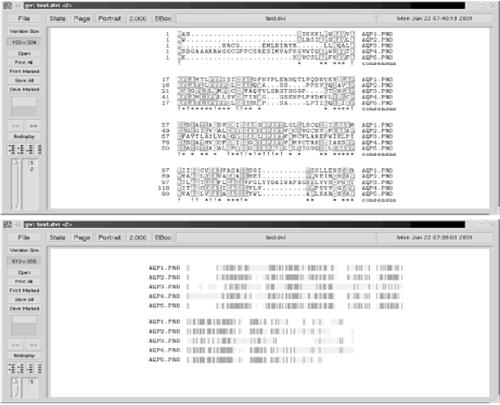
14.3.2 Viewing Sequence Distances Geometrically
Multiple sequence alignments and sequence logos represent similarities at every position of a group of aligned sequences. However, even with coloring of conserved residues, it isn't always easy to tell how the sequences are related. Sometimes, it's useful to look at an even higher level of abstraction to see how the sequences cluster. Phylogenetic trees represent one way to visualize relatedness.
DGEOM, a set of programs by Mark J. Forster and coworkers, takes a set of aligned sequences (either a multiple sequence alignment in GCG's MSF format, or a set of pairwise alignments) and represents them as points in a 3D space, where the distances between the points represent the evolutionary distances between the sequences. The points are written to a PDB file and can be viewed with your choice of protein structure viewers. Some may flinch at the idea of storing a representation of a sequence alignment in a file format intended to store structural data, but the program works well, and since high-quality structure visualization packages are easy to find, this approach avoids the need for a standalone graphics system. The programs are written in Perl and C, making them fairly easy to modify.
Another implementation of the geometric approach to viewing sequence relationships is the SeqSpace package developed by Chris Dodge and Chris Sander at the EBI. This package includes C++ programs for computing the sequence distances, and it uses Java viewers to render the points in 3D.
14.4 Networks and Pathway Visualization
As of this writing, there is no standard package for visualizing interactions between molecules in a pathway or network. The most common way to represent molecular interactions schematically is in the form of a graph.[3] Graphs can also be useful for illustrating other data that represents interactions, including the output of cluster analyses and interacting residues in protein structures. Biological networks, such as metabolisms and signaling pathways, tend to be very densely connected, and creating readable, highly connected graphs isn't an easy task. Fortunately, AT&T Research distributes GraphViz (https://www.research.att.com/sw/tools/graphviz/), a freely available suite of programs that allow you to draw and edit graphs. This package has three features that make it particularly attractive: it runs quickly, it has excellent documentation, and it uses a flexible and intuitive syntax to describe graphs.
Here we are talking about the graph theory kind of graph, in which a set of dots (nodes) are connected by a set of lines (edges). Directed graphs are those in which the edge connecting two nodes has a direction. Edges in directed graphs are usually represented using arrows pointing in the direction of a connection. In an undirected graph, the edges have no direction.
The GraphViz package consists of five programs:
dot
Draws directed graphs
neato
Draws undirected graphs
dotty
A graphical interface for editing graphs
lefty
A language for editing graphs and other diagrams; used to write dotty
tcldot
A graphical interface to dot written in the Tcl language
To draw a directed graph of a small set of interactions, you can type the following code into a text editor and save it to a file named morphopath.dot:
digraph G
The dot program is invoked using the following command at the shell prompt:
% dot -Tps morphopath.dot -o morphopath.ps end
This command tells the dot program in the GraphViz suite to produce a PostScript image of the graph described by morphopath.dot and to put the image in the file morphopath.ps (see Figure 14-2).
Figure 14-2. morphopath pathway output
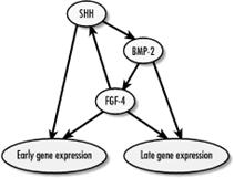
If you have some experience with the C programming language, you might recognize the similarity of the graph description format to a struck in C. This structured approach to describing the graph's layout makes it possible to define graphs within graphs, and also makes it straightforward to generate GraphViz files from Perl scripts. In addition to specifying connectivity, graphs produced by the GraphViz programs can be annotated with labels, different arrow types, and highlighted boxes.
14.5 Working with Numerical Data
Numerical data can always be fed into a spreadsheet program such as Microsoft Excel or StarOffice Calc and plotted using the program's built-in graphing functions. Often, this is the best way to make plots quickly. However, you will encounter situations in which you need more control over the plotting process than the spreadsheet provides. Two common examples of this kind of situation are in formatting your plots for publication and in dealing with high-dimensional data sets. If you do have to create figures from your data, we encourage you to take a look at Edward Tufte's books on visual explanations (see the Bibliography). They are full of examples and tips on making clean figures that clearly say what you mean.
In this section, we describe some programs that can create plots. In addition, we introduce two special-purpose programming languages that include good facilities for visualization as well as data analysis: the statistics language R (and its commercial cousin, S-plus) and the numerical programming language Matlab (and its free counterpart, Octave).
14.5.1 gnuplot and xgfe
gnuplot (https://www.gnuplot.org) is one of the more widely used programs for producing plots of scientific data. Because of its flexibility, longevity, and open source nature, gnuplot is loaded with features, including scripting and facilities for including plots in documents. The dark side of this flexibility and longevity, though, is a fairly intimidating command syntax. Fortunately, a graphical interface to gnuplot called xg fe exists. xg fe is good for quickly plotting either data or a function, as shown in Figure 14-3. You can find out more about xg fe at https://home.flash.net/~dmishee/xgfe/xgfe.html.
Figure 14-3. Output from xg fe/gnuplot
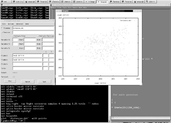
If you need to exert more control over the format of the output, though, it behooves you to read through the gnuplot documentation and see what it can do. Additionally, if you need to aumotically generate many plots from data, you may want to figure out how to control gnuplot 's behavior using Perl or another scripting language.
14.5.2 Grace: The Pocketknife of Data Visualization
Grace (https://plasma-gate.weizmann.ac.il/Grace/)Error! Hyperlink reference not valid.and its predecessor, xmgr, are alternatives to gnuplot as a fairly powerful tool for plotting 2D data. Grace uses a simple graphical interface under the X Window System, which allows a fair amount of menu-driven customization of plots. Like xg fe, Grace provides the fairly simple 20% functionality you need 80% of the time. In addition to its current main distribution site at the Weizmann Institute of Science in Israel (which always has the latest version), there are a number of mirror sites from which Grace can be acquired. The home site also has a useful FAQ and tutorial introduction to working with Grace.
14.5.3 Multidimensional Analysis: XGobi and XGvis
Plotting programs such as Grace and gnuplot work well if your data has two or three variables that can be assigned to the plot axes. Unfortunately, most interesting data in biology has a much higher dimensionality. The science of investigating high-dimensional data is known as multivariate or multidimensional analysis. One significant problem in dealing with multidimensional data is visualization. For those who can't envision an 18-dimensional space, there is XGobi (https://www.research.att.com/areas/stat/xgobi/). XGobi and XGvis are a set of programs freely available from AT&T Labs. XGobi allows you to view data with many variables three dimensions at a time as a constellation of points you can rotate using a mouse. XGvis performs multidimensional scaling, the intelligent squashing of high-dimensional data into a space you can visualize (usually a 2D plot or a rotatable 3D plot). Figure 14-4 shows output from XGobi.
Figure 14-4. Screenshot from XGobi
XGobi has a huge number of features; here is a brief explanation to get you started. XGobi takes as input a text file containing columns of data. If you have a datafile named xgdemo.dat, it can be viewed in XGobi by typing the following command at the shell prompt:
% xgobi xgdemo.dat &
XGobi initially presents the points in a 2D scatterplot. Selecting Rotation from the View menu at the top of the window shows a moving 3D plot of the points that you can control with the mouse by clicking within the data points and moving the mouse. Selecting Grand Tour or Correlation Tour from the View menu rotates the points in an automated tour of the data space.
The variable widgets (the circles along the right side of the XGobi interface) represent each of the variables in the data. The line in each widget represents the orientation of that variable's axis in the plot. If the data contains more than three variables, you can select the variables to be represented by clicking first within the widget of the variable you want to dismiss, and then within the widget of the variable to be displayed. Finally, clicking on the name of the corresponding variable displays a menu of transformations for that axis (e.g., natural logarithms, common logs, squares, and square roots). Like the GraphViz graph drawing programs, XGobi and XGvis are superbly documented and easy to install on Linux systems if you follow the instructions on the XGobi home page. Some Linux distributions (such as SuSE) even include XGobi.
14.5.4 Programming for Data Analysis
In this section, we introduce two new programming languages that are well adapted for data analysis. The proposition of learning more languages after just learning Perl may seem a little perverse. Who would want to learn a whole language just to do data analysis? If your statistics requirements can be satisfied with a spreadsheet and calculator, these packages may not be for you. Also, as we saw in the last chapter, there are facilities for creating numerically sophisticated applications using Perl, particularly the PDL.
However, many problems in bioinformatics require the use of involved numerical or statistical calculations. The time required to develop and debug such software is considerable, and it may not be worth your time to work on such code if it's used only once or twice. Fortunately, in the same way that Perl makes developing data-handling programs easy, data analysis languages (for lack of a better term) ease the prototyping and rapid development of data analysis programs. In the next sections, we introduce R (and its commercial cousin, S-plus), a language for doing statistics; and Matlab (and its free cousin, Octave), a language for doing numerical mathematics.
14.5.4.1 R and S-plus
R is a free implementation of the S statistics programming language developed at AT&T Bell Laboratories. R was developed by Ross Ihaka and Robert Gentleman at the University of Auckland. Both R and its commercial cousins (S-plus 3.x, 4.x, and 2000) are available for the Unix and Win32 platforms, and both have a syntax that has been described as 'not dissimilar,' so we use R to refer to both languages.
R is usually run within an interpreted environment. Instead of writing whole programs that are executed from the command line, R provides its own interactive environment in which statements can be run one at a time or as whole programs. To start the R environment, type in R at the command prompt and hit the Enter key. You should see something like this:
R : Copyright 2000, The R Development Core Team
Version 1.1.1 (August 15, 2000)
R is free software and comes with ABSOLUTELY NO WARRANTY.
You are welcome to redistribute it under certain conditions.
Type '?license' or '?licence' for distribution details.
R is a collaborative project with many contributors.
Type '?contributors' for a list.
Type 'demo( )' for some demos, 'help( )' for on-line help, or
'help.start( )' for a HTML browser interface to help.
Type 'q( )' to quit R.
The angle bracket (>) at the bottom of this screen is the R prompt, similar to the shell prompt in Unix. In the following examples, we write the R prompt before the things that the user (that's you) is supposed to type.
Before anything else, you should know two commands. Arguably, the most important command in any interactive environment is the one that lets you exit back out to the operating system. In R, the command to quit is:
> q( )
The second most useful command is the one that provides access to R's online help system, help( ). The default help( ) command, with no arguments, returns an explanation of how to use help( ). If you want help on a specific R function, put the name of the function in the parentheses following help. So, for example, if you want to learn how the source( )function works, you can type:
> help(source)
You can also use ? as shorthand for help( ). So, instead of typing help (source) in the example, you can just enter ?source.
As mentioned earlier, the R environment is interactive. If you type the following:
> 2 + 2
R tells you that two plus two does, in fact, equal four:
> 2 + 2
The R response (4 ) is preceded by a bracketed number ([1] ), which indicates the position of the answer in the output vector. Unlike Perl, R has no scalar variables. Instead, single numbers like the previous answer are stored in a vector of length one. Also, note that the first element in the vector is numbered 1 instead of 0.[4]
Actually, R vectors do have a zero element, but it doesn't accept values assigned to it, and it returns numeric(0), which is an empty vector.
The <- operator is used as the assignment operator. Its function is similar to the = operator in Perl. Typing:
> a <- 2 + 2
produces no output, since the result of the calculation is stored in the variable on the left side of the assignment operator. In order to see what value a variable contains, enter its name at the R prompt:
> a <- 2 + 2
> a
Just as Perl has basic datatypes that are useful for working with text, R has datatypes that are useful for doing statistics. We have already seen the vector; R also has matrices, arrays (which are a multidimensional generalization of matrices), and factors (lists of strings that label vectors of the same length).
14.5.4.2 Online resources for R
The place to go for more information on R is the Comprehensive R Archive Network (CRAN). You can find the CRAN site nearest to you either by using your favorite search engine or off a link from the R Project home page (https://www.R-project.org). CRAN has a number of packages for specific statistical applications implemented in R and available as RPM files (for information on installing RPMs, see Chapter 3). If your project requires sampling, clustering, regression, or factor analysis, R can be a lifesaver. R can even be made to directly access XGobi as an output system, so that the results of your computations can be plotted in two or more dimensions.
You can try R without having to install it, thanks to Rweb (https://www.math.montana.edu/Rweb/), a service provided by the Montana State University Mathematics Department. Rweb accepts your R code, runs it, and returns a page with the results of the calculation. If you want to use R for anything beyond simple demonstrations, though, it's faster to download the RPM files and run R on a local computer.
If you find that R is useful in your work, we vigorously recommend you supplement the R tutorial, An Introduction to R, and the R FAQ (https://cran.r-project.org/) with the third edition of Modern Applied Statistics with S-Plus (see the Bibliography). Both Venables and Ripley are now part of the R development core team, and although their text is primarily an S-plus book, supplements are available from Ripley's web site (https://www.stats.ox.ac.uk/~ripley/)that make the examples in book more easily used under R.
14.5.4.3 Matlab and Octave
GNU Octave (https://www.gnu.org/software/octave/octave.html) is a freely available programming language whose syntax and functions are similar to Matlab, a commercial programming environment from The MathWorks, Inc. (https://www.mathworks.com/products/matlab/). Matlab is popular among engineers for quickly writing programs that perform large numbers of numerical computations. Octave (or Matlab) is worth a look if you want to write quick prototypes of number-crunching programs, particularly for data analysis or simulation. Both Octave and Matlab are available for Unix and Windows systems. Octave source code, binaries, and documentation are all available online; they are also distributed as part of an increasing number of Linux distributions.
Octave produces graphical output using the gnuplot package mentioned previously. While this arrangement works well enough, it is rather spartan compared to the plotting capabilities of Matlab. In fact, if you are a student, we will take off our open source hats and strongly encourage you to take advantage of the academic pricing on Matlab; it will add years to your life. As a further incentive, a number of the data mining and machine learning tools discussed in the next section are available as Matlab packages
14.6 Visualization: Summary
This section has described solutions to data presentation problems that arise frequently in bioinformatics. For some of the most current work on visualization in bioinformatics, see the European Bioinformatics Institute's visualization information off the Projects link on their industrial relations page (https://industry.ebi.ac.uk). Links to more online visualization and data mining resources are available off the web page for this book. Table 14-1 shows the tools and techniques that are used for data visualization.
Table 14-1. Data Visualization Tools and Techniques
|
What you do |
Why you do it |
What you use to do it |
|
View graphics files |
To view results and check figures |
xzgv |
|
View PDF or PostScript files |
To read articles in electronic form |
gv, Adobe Acrobat Reader |
|
Manipulate graphics files |
For preparation of figures |
The GIMP |
|
Plot data in two or three dimensions |
To summarize data for presentations |
Grace, gnuplot |
|
Multidimensionalvisualization |
To explore data with more than three variables |
XGobi |
|
Multidimensional scaling |
To view high-dimensional data in2D or 3D |
XGvis |
|
Plot graphical structures |
To draw networks and pathways |
GraphViz programs |
|
Print sequence alignment clearly |
To format sequence alignment for publication |
TEXshade |
|
Statistics-heavy programming for data analysis |
For rapid prototyping of statistical data-analysis tools |
R (or S-plus) |
|
Numerically intensive programming for data analysis |
For rapid prototyping of tools that make heavy use of matrices |
GNU Octave (or Matlab) |
14.7 Data Mining and Biological Information
One of the most exciting areas of modern biology is the application of data mining methods to biological databases. Many of these methods can equally well fall into the category of machine learning, the name used in the artificial intelligence community for the larger family of programs that adapt their behavior with experience. We present here a summary of some techniques that have appeared in recent work in bioinformatics. The list isn't comprehensive but will hopefully provide a starting point for learning about this growing area.
A word of caution: anthropomorphisms have a tendency to creep into discussions of data mining and machine learning, but there is nothing magical about them. Programs are said to 'learn' or be 'trained,' but they are always just following well-defined sets of instructions. As with any of the tools we've described in this book, data mining tools are supplements, rather than substitutes, for human knowledge and intuition. No program is smart enough to take a pile of raw data and generate interesting results, much less a publication-quality article ready for submission to the journal of your choice. As we've stressed before, the creation of a meaningful question, the experimental design, and the meaningful interpretation of results are your responsibility and yours alone.
14.7.1 Problems in Data Mining and Machine Learning
The topics addressed by data mining are ones that statisticians and applied mathematicians have worked on for decades. Consequently, the division between statistics and data mining is blurry at best. If you do work with data mining or machine learning techniques, you will want to have more than a passing familiarity with traditional statistical techniques. If your problem can be solved by the latest data-mining algorithm or a straightforward statistical calculation, you would do well to choose the simple calculation. By the same token, please avoid the temptation to devise your own scoring method without first consulting a statistics book to see if an appropriate measure already exists. In both cases, it will be easier to debug and easier to explain your choice of a standard method over a nonstandard one to your colleagues.
14.7.1.1 Supervised and unsupervised learning
Machine learning methods can be broadly divided into supervised and unsupervised learning. Learning is said to be supervised when a learning algorithm is given a set of labeled examples from which to learn (the training set) and is then tested on a set of unlabeled examples (the test set). Unsupervised learning is performed when data is available, but the correct labels for each example aren't known. The objective of running the learning algorithm on the data is to find some patterns or trends that will aid in understanding the data. For example, the MEME program introduced in Chapter 8, performs unsupervised learning in order to find sequence motifs in a set of unaligned sequences. It isn't known ahead of time whether each sequence contains the pattern, where the pattern is, or what the pattern looks like.
Cluster analysis is another kind of unsupervised learning that has received some attention in the analysis of microarray data. Clustering, as shown in Figure 14-5, is the procedure of classifying data such that similar items end up in the same class while dissimilar items don't, when the actual classes aren't known ahead of time. It is a standard technique for working with multidimensional data. Figure 14-5 shows two panels with unadorned dots on the left and dots surrounded by cluster boundaries on the right.
Figure 14-5. Clustering
14.7.2 A Collection of Data Mining Techniques
In this section, we describe some data mining methods commonly reported in the bioinformatics literature. The purpose of this section is to provide an executive summary of the complex tricks for data analysis. You aren't expected to be able to implement these algorithms in your programming language of choice. However, if you see any of these methods used to analyze data in a paper, you should be able to recognize the method and, if necessary, evaluate the way in which it was applied. Like any technique in experimental biology, it is important to have an understanding of the machine learning methods used in computational biology to know whether or not they have been used appropriately and correctly.
14.7.2.1 Decision trees
In its simplest form, a decision tree is a list of questions with yes or no answers, hierarchically arranged, that lead to a decision. For instance, to determine whether a stretch of DNA is a gene, we might have a tree like the one shown in Figure 14-6.
Figure 14-6. Simple gene decision tree
A tree like this one is easy to work through, since it has a finite number of possibilities at each branch, and any path through the tree leads to a decision. The structure of the tree and the rules at each of the branches are determined from the data by a learning algorithm. Techniques for learning decision trees were described by Leo Breiman and coworkers in the early 1980s, and were later popularized in the machine learning community by J. R. Quinlan, whose freely available C4.5 decision tree software and its commercial successor, C5, are standards in the field.
One major advantage of decision trees over other machine learning techniques is that they produce models that can be interpreted by humans. This is an important feature, because a human expert can look at a set of rules learned by a decision tree and determine whether the learned model is plausible given real-world constraints.[5] In biology, tree classifiers tend to be used in pattern recognition problems, such as finding gene splice sites or identifying new occurrences of a protein family member. The MORGAN genefinder developed by Steven Salzberg and coworkers is an example of a decision tree approach to genefinding.
The canonical decision-tree urban legend comes from an application of trees by a long-distance telephone company that wanted to learn about churn, the process of losing customers to other long-distance companies. They discovered that an abnormally large number of their customers over the age of 70 were subject to churn. A human recognized something the program did not: humans can die of old age. So, being able to interpret your results can be useful.
14.7.2.2 Neural networks
Neural networks are statistical models used in pattern recognition and classification. Originally developed in the 1940s as a mathematical model of memory, neural networks are sometimes also called connectionist models because of their representation as nodes (which are usually variables) connected by weighted functions. Figure 14-7 shows the process by which a neural network is constructed. Please note, though, that there is nothing particularly 'neural' about these models, nor are there actually physical nodes and connections involved. The idea behind neural networks is that, by working in concert, these simple processing elements can perform more complex computations.
Figure 14-7. Neural network diagram
A neural network is composed of a set of nodes that are connected in a defined topology, where each node has input and output connections to other nodes. In general, a neural network will receive an input pattern (for example, an amino acid sequence whose secondary structure is to be predicted), which sets the values of the nodes on the first layer (the input layer). These values are propagated according to transfer functions (the connections) to the next layer of nodes, which propagate their values to the next layer, until the output layer is reached. The pattern of activation of the output layer is the output of the network. Neural networks are used extensively in bioinformatics problems; examples include the PHD (https://www.embl-heidelberg.de/predictprotein/predictprotein.html) and PSIPRED (https://insulin.brunel.ac.uk/psipred/) secondary structure predictors described in Chapter 9, and the GRAIL genefinder (https://compbio.ornl.gov/grailexp/) mentioned in Chapter 7.
14.7.2.3 Genetic algorithms
Genetic algorithms are optimization algorithms. They search a large number of possible solutions for the best one, where 'best' is determined by a cost function or fitness function. Like neural networks, these models were inspired by biological ideas (in this case, population genetics), but there is nothing inherently biological about them. In a genetic algorithm, a number of candidate solutions are generated at random. These candidate solutions are encoded as chromosomes. Parts of each chromosome are then exchanged à la homologous recombination between real chromosomes. The resulting recombined strategies are then evaluated according to the fitness function, and the highest scoring chromosomes are propagated to the next generation. This recombination and propagation loop continues until a suitably good solution is found. Genetic algorithms are frequently used in molecular simulations, such as docking and folding of proteins.
14.7.2.4 Support vector machines
In late 1998, a machine learning tool called the support vector machine (SVM) began to attract a great deal of attention in bioinformatics. Support vector machines were developed by Vladimir Vapnik of Bell Laboratories, an early pioneer of machine learning methods. They have been applied to a wide range of problems, from optical character recognition to financial time series analysis and recognizing spam (the email variety, not the lunch meat). SVMs were first applied to biological problems by Tommi Jaakola (now at MIT), David Haussler, and coworkers at UC Santa Cruz, who used them for protein sequence classification. They have since been applied to many of the standard computational biology challenge problems (function prediction, structure prediction, and genefinding) but have gained the most attention for their use in microarray analysis.
Support vector machines are supervised classifiers that try to find a linear separation between different classes of points in a high-dimensional space. In a 2D space, this separator is a line; in 3D, it's a plane. In general, this separating surface is called a hyperplane. Support vector machines have two special features. First, instead of just finding any separating hyperplane, they are guaranteed to find the optimal one, or the one whose placement yields the largest separation between the two classes. The data points nearest the frontier between the two classes are called the support vectors.[6] Second, although SVMs are linear classifiers, they can classify nonlinearly separable sets of points by transforming the original data points into a higher dimensional space in which they can be separated by a linear surface.
Vectors, in this case, refer to the coordinates of the data points. For example, on a 2D map, you might have pairs of (x,y) coordinates representing the location of the data points. These ordered pairs are the vectors.
Table 14-2 shows some of the most popular data-mining tools and techniques.
Table 14-2. Data Mining Tools and Techniques
|
What you do |
Why you do it |
What you use to do it |
|
Clustering |
To find similar items when a classification scheme isn't known ahead of time |
Clustering algorithms, self-organizing maps |
|
Classification |
To label each piece of data according to a classification scheme |
Decision trees, neural networks, SVMs |
|
Regression |
To extrapolate a trend from a few examples |
Regression algorithms, neural networks, SVMs, decision trees |
|
Combining estimators |
To improve reliability of prediction |
Voting methods, mixture methods |
Bibliography
Biblio.1 Unix
Learning Red Hat Linux and Learning Debian GNU Linux. B. McCarty. O'Reilly & Associates. Good introductory guides to setting up systems with these releases of Linux.
Learning the Unix Operating System. J. Peek, G. Todino, and J. Strang. O'Reilly & Associates. A concise introduction to Unix for the beginner.
The Linux Desk Reference. S. Hawkins and J. Brockmeier. Prentice Hall.
Linux in a Nutshell. Siever, et al. O'Reilly & Associates. A no-nonsense quick-reference guide to Linux commands.
Running Linux. M. Welsh and L. Kaufman. O'Reilly & Associates. A relatively comprehensive how-to guide for setting up a Linux system.
Unix for the Impatient. P. Abrahams and B. Larson. Addison Wesley. A detailed yet user-friendly presentation of everything a Unix user needs to know. (My first and still favorite Unix guide. CJG)
Unix in a Nutshell. A. Robbins. O'Reilly & Associates. A no-nonsense quick-reference guide to Unix commands.
Biblio.2 SysAdmin
Essential System Administration. A. Frisch. O'Reilly & Associates. A detailed guide to administration of Unix systems.
Using csh & tcsh. P. DuBois. O'Reilly & Associates. A detailed guide to using two of the most common shell environments.
Biblio.3 Perl
Elements of Programming in Perl. A. L. Johnson. Manning Publications. Good introduction to Perl as a first programming language
Learning Perl. R. Schwartz and T. Christiansen. O'Reilly & Associates. Introduction to Perl but assumes prior experience with another programming language.
For a more detailed, biology-oriented Perl tutorial, we recommend the one available online at Lincoln Stein's laboratory page at Cold Spring Harbor Labs, https://stein.cshl.org.
Mastering Algorithms in Perl. J. Orwant, J. Hietaniemi, and J. Macdonald. O'Reilly & Associates. Both this book and the next cover interesting things that can be done with Perl.
Perl Cookbook. T. Christiansen and N. Torkington. O'Reilly & Associates.
Programming Perl. L. Wall, T. Christiansen, and J. Orwant. O'Reilly & Associates. The bible of Perl.
Biblio.4 General Reference
Finding Out About: Search Engine Technology from a Cognitive Perspective. R. Belew. Cambridge University Press. A fascinating discussion of information retrieval and the process of web-based research from a cognitive science perspective. Both practical and philosophical aspects are covered.
All three of the following books cover general programming techniques:
Code Complete. S. McConnell. Microsoft Press.
The Practice of Programming. B. W. Kernighan and R. Pike. Addison Wesley
Programming Pearls. J. Bentley. Addison Wesley
Biblio.5 Bioinformatics Reference
Bioinformatics: A Machine Learning Approach. P. Baldi and S. Brunak. MIT Press. The authors have firsthand experience with applying neural networks and hidden Markov models to sequence analysis, including genefinding, DNA feature detection, and protein family modeling.
Bioinformatics: A Practical Guide to the Analysis of Genes and Proteins. A. D. Baxevanis and B. F. F. Ouellette. John Wiley & Sons. A gentle introduction to biological information and bioinformatics tools on the Web, focused on NCBI tools.
Biological Sequence Analysis: Probabilistic Models of Proteins and Nucleic Acids. R. Durbin, S. Eddy, A. Krogh, and G. Mitchison. Cambridge University Press. A rigorous presentation of the statistical and algorithmic basis of sequence analysis methods, including pairwise and multiple sequence analysis, motif discovery, and phylogenetic analysis.
Molecular Systematics. D. M. Hillis, C. Moritz, and B. K. Mable, Eds. Sinauer and Associates. Although the first two-thirds of the book are devoted to experimental methods, the chapters on the methods for inferring and applying phylogenies provide a rigorous and comprehensive follow-up to the Graur and Li book.
Biblio.6 Molecular Biology/Biology Reference
Fundamentals of Molecular Evolution. D. Graur, W-H. Li. Sinauer and Associates. A readable explanation of the mechanisms by which genomes change over time, with a discussion of phylogenetic inference based on molecular data.
Molecular Systematics. D. M. Hillis, C. Moritz, and B. K. Mable, eds. Sinauer and Associates. Although the first two-thirds of the book are devoted to experimental methods, the chapters on the methods for inferring and applying phylogenies provide a rigorous and comprehensive follow-up to the Graur and Li book.
Biblio.7 Protein Structure and Biophysics
Intermolecular and Surface Forces. J. Israelachvili. Academic Press. A must-have book for any serious student of macromolecular structure and molecular biophysics. This book details the physical chemistry of interactions among molecules and between molecules and surfaces.
Introduction to Protein Structure. C-I. Branden and J. Tooze. Garland Publishing. An illustrated guide to the basic principles of protein structure and modeling.
Biblio.8 Genomics
Genomes. T. A. Brown. Wiley-Liss. A thorough presentation of molecular genetics from the genomics perspective.
Genomics: The Science and Technology Behind the Human Genome Project. C. R. Cantor and C. L. Smith. John Wiley & Sons. If you want to understand, in detail, how genomic sequence data is obtained, this is the book to have. It exhaustively details experimental protocols for sequencing and mapping and explores the future of sequencing technology.
Biblio.9 Biotechnology
DNA Microarrays: A Practical Approach. M. Schena, ed. Oxford University Press. An introduction to the basics of DNA microarray technology and its applications.
Proteome Research: New Frontiers in Functional Genomics. M. R. Wilkins, K. L. Williams, R. D. Appel, and D. F. Hochstrasser, eds. Springer. An introduction to new techniques for protein identification and analysis, from 2D-PAGE to MALDI-TOF and beyond.
Biblio.10 Databases
CGI Programming with Perl. S. Guelich, S. Gundavaram, and G. Birznieks. O'Reilly & Associates. An introduction to the CGI protocol for generating active-content web pages. If you are interested in web software development, this book is an essential starting point.
Joe Celko's Data and Databases: Concepts in Practice. J. Celko. Morgan Kaufman. A good introduction to relational database concepts and the use of SQL.
MySQL. P. DuBois. New Riders. A detailed guide to using MySQL. Detailed coverage of administration and security issues.
MySQL & mSQL. R. J. Yarger, G. Reese, and T. King. O'Reilly & Associates. An introduction to using MySQL and mSQL; also contains an introduction to RDB concepts and database normalization. O'Reilly also publishes a collection of reference books about Oracle, if you prefer to start using Oracle from the beginning.
Biblio.11 Visualization
Understanding Robust and Exploratory Data Analysis. D. C. Hoaglin, et al. eds. John Wiley & Sons. A classic book on visualization techniques. Don't be put off by the fact that the focus of the book is on techniques for doing analysis by hand rather than the latest computational tricks: the methods described are implemented in many visualization packages and are easily applicable to the latest bioinformatics problems.
The Visual Display of Quantitative Information, Envisioning Information, and Visual Explanations. E Tufte. Graphics Press. In each book, Tufte illustrates good and bad practices in visual data analysis using examples from newspapers, advertising campaigns, and train schedules (to name a few).
The Visualization Toolkit: An Object-Oriented Approach to 3-D Graphics. W. Schroeder, K. Martin, and B. Lorensen. Prentice Hall Computer Books. For those readers who want a more active role in designing visualization tools, this book combines introductions to computer graphics and visualization practices with a description of a working implementation of a complete visualization system, the Visualization Toolkit (VTK). VTK is an object-oriented, scriptable framework for building visualization tools. It is available from https://www.kitware.com.
Biblio.12 Data Mining
Data Mining: Practical Machine Learning. I. Witten and E. Frank. Morgan Kaufman. A clearly written introduction to data mining methods. It comes with documentation for the authors' WEKA program suite, a set of data mining tools written in Java that can be freely downloaded from their web site.
Data Preparation for Data Mining. D. Pyle. Morgan Kaufman. For readers looking for more insight into the data-preparation process.
Machine Learning. T. Mitchell. McGraw-Hill. Provides a complementary treatment of the same methods as the previous book and is more formal but no less practical.
Modern Applied Statistics with S-Plus. Brian D. Ripley and William N. Venables. Springer Verlag.
Numerical Recipes in C. W. H. Press, S. A. Teukolsky, W. T. Vetterling, and B. P. Flannery. Cambridge University Press. A comprehensive introduction to the techniques that underlie all nontrivial methods for data analysis. Combines mathematical explanations with efficient C implementations. In addition to the hardcopy form, the entire book and all its source code are available online at no charge from https://www.nr.com.
Colophon
Our look is the result of reader comments, our own experimentation, and feedback from distribution channels. Distinctive covers complement our distinctive approach to technical topics, breathing personality and life into potentially dry subjects.
The animal on the cover of Developing Bioinformatics Computer Skills is Caenorhabditis elegans, a small nematode worm. Unlike many of its nastier parasitic cousins, C. elegans lives in the soil where it feeds on microbes and bacteria. It grows to about 1 mm in length.
In spite of its status as a 'primitive' organism, C. elegans shares with H. sapiens many essential biological characteristics. C. elegans begins life as a single cell that divides and grows to form a multicellular adult. It has a nervous system and a brain (more properly known as the circumpharyngeal ring) and a muscular system that supports locomotion. It exhibits behavior and is capable of rudimentary learning. Like humans, it comes in two sexes, but in C. elegans those sexes consist of a male and a self-fertilizing hermaphrodite. C. elegans is easily grown in large numbers in the laboratory, has a short (2-3 week) lifespan, and can be manipulated in sophisticated experiments. These characteristics make it an ideal organism for scientific research.
The C. elegans hermaphrodite has 959 cells, 300 of which are neurons, and 81 of which are muscle cells. The entire cell lineage has been traced through development. The adult has a number of sensory organs in the head region which respond to taste, smell, touch, and temperature. Although it has no eyes, it does react slightly to light. C. elegans has approximately 17,800 distinct genes, and its genome has been completely sequenced. Along with the fruit fly, the mouse, and the weed Arabidopsis, C. elegans has become one of the most studied model organisms in biology since Sydney Brenner first focused his attention on it decades ago.
Mary Anne Weeks Mayo was the production editor and copyeditor for Developing Bioinformatics Computer Skills. Rachel Wheeler proofread the book. Linley Dolby and Sheryl Avruch provided quality control. Gabe Weiss, Edie Shapiro, Matt Hutchinson, and Sada Preisch provided production assistance. Joe Wizda wrote the index.
Ellie Volckhausen designed the cover of this book, based on a series design by Edie Freedman. The cover image is an original illustration created by Lorrie LeJeune, based on a photograph supplied by Leon Avery at the University of Texas Southwestern Medical Center. Emma Colby produced the cover layout with QuarkXPress 4.1 using Adobe's ITC Garamond font.
Melanie Wang designed the interior layout based on a series design by Nancy Priest. Cliff Dyer converted the files from MSWord to FrameMaker 5.5 using tools created by Mike Sierra. The text and heading fonts are ITC Garamond Light and Garamond Book; the code font is Constant Willison. The illustrations for this book were created by Robert Romano and Lucy Muellner using Macromedia Freehand 9 and Adobe Photoshop 6. This colophon was written by Lorrie LeJeune.
|
Politica de confidentialitate | Termeni si conditii de utilizare |

Vizualizari: 55338
Importanta: ![]()
Termeni si conditii de utilizare | Contact
© SCRIGROUP 2025 . All rights reserved