| CATEGORII DOCUMENTE |
| Bulgara | Ceha slovaca | Croata | Engleza | Estona | Finlandeza | Franceza |
| Germana | Italiana | Letona | Lituaniana | Maghiara | Olandeza | Poloneza |
| Sarba | Slovena | Spaniola | Suedeza | Turca | Ucraineana |
Data Mining
Introduction to Data Mining
Organizations worldwide generate large amount of data that is mostly unorganized. This unorganized data requires processing to be done to generate meaningful and useful information. In order to organize large amount of data, it is necessary to implement the concept of database management systems such as Oracle and SQL Server. These database management systems require usage of SQL, a specialized query language to retrieve data from a database. However, the use of SQL is not always adequate to meet the end user requirements of specialized and sophisticated information from an unorganized large data bank. This requires looking for certain alternative techniques to retrieve information from large and unorganized source of data.
Following chapters introduce the basic concepts of data mining, a specialized data processing technique. These chapters explore the various tasks, models, and techniques that are used in data mining in order to retrieve meaning and useful information from large and unorganized data.
What is Data Mining?
Data Mining is well known as Knowledge Discovery in Databases.
Data mining is the technique of extracting meaningful information from large and mostly unorganized data banks. It is the process of performing automated extraction and generation predictive information from large amount of data. It enables user to understand the current market trends and enables you to take proactive measures to gain maximum benefit from the same.
The data mining process uses a variety of analysis tools to determine the relationships between data in the data banks and use the same to make valid predictions. Data mining is the integration of various techniques from multiple disciplines such as statistics, machine learning, pattern recognition, neural networks, image processing, and database management systems and so on.
The Data Mining Process
Data mining operations require a systematic approach. The process of data mining is generally specified in the form of an ordered list but the process is not linear, sometimes is necessary to step back and rework on the previously performed step.
The
general phases in the data mining process to extract knowledge as shown on ![]() are:
are:
1. Problem definition
This phase is to understand the problem and the domain environment in which the problem occurs. The problem has to be clearly defined before proceeding further. Problem definition specifies the limits within which the problem needs to be solved. It also specifies the cost limitations to solve the problem.
2. Creating a database for data mining
This phase is to create a database where the data to be mined are stored for knowledge acquisition. Creating a database does not require creation specialized database management system. You can even use a flat file or a spreadsheet to store data. Data warehouse is also a kind of data storage where large amount of data is stored for data mining. The creation of data mining database consumes about 50% to 90% of the overall data mining process.
3. Exploring the database
This phase is to select and examine important data sets of a data mining database in order to determine their feasibility to solve the problem. Exploring the database is a time-consuming process and requires a good user interface and computer system with good processing speed.
4. Preparation for creating a data mining model
This phase is to select variables to act as predictors. New variables are also built depending upon the existing variables along with defining the range of variables in order to support imprecise information.
5. Building a data mining model
This phase is to create multiple data mining models and to select the best of these models. Building a data mining model is an interactive process. At times, user needs to go back to the problem definition phase in order to change the problem definition itself. The data mining model that the user selects can be a decision tree, an artificial neural network, or an association rule model.
6. Evaluating the data mining model
This phase is to evaluate the accuracy of the selected data mining model. In data mining, the evaluating parameter is data accuracy in order to test the working of the model. This is because the information generated in the simulated environment varies from the external environment. The errors that occur during the evaluation phase needs to be recorded and the cost and time involved in rectifying the error needs to be estimated. External validation is also needs to be performed in order to check whether the selected model performs correctly when provided real world values.
7. Deploying the data mining model
This phase is to deploy the built and the evaluated data mining model in the external working environment. A monitoring system should monitor the working of the model and generate reports about its performance. The information in the report helps enhance the performance of selected data mining model.
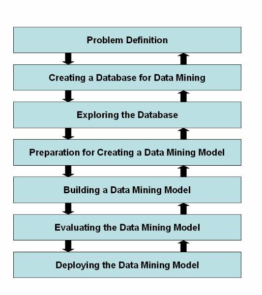
Figure 1.2-1 Life Cycle of the Data Mining Process
Data Mining Tasks
Data mining makes use of various algorithms to perform a variety of tasks. These algorithms examine the sample data of a problem and determine a model that fits close to solving the problem. The models that user determines to solve a problem are classified as predictive and descriptive.
A predictive model enables to the user to predict the values of data by making use of known results from a different set of sample data. The data mining tasks that form the part of the predictive model are:
Classification
Regression
Time series analysis
A descriptive model enables you to determine the patterns and relationships in a sample data. The data mining tasks that form the part of the descriptive model are:
Clustering
Summarization
Association rules
Sequence discovery
Classification
Classification is an example of data mining task that fits in the predictive model of data mining. The use of classification task enables the user to classify data in a large data bank into predefined set of classes. The classes are defined before studying or examining data in the data bank. Classification tasks not only enable the user to study and examine the existing sample data but also enable him to predict the future behaviour of that sample data.
Example: The fraud detection in credit card related transaction, text document analysis, and probability of an employee to leave an organization are some of the tasks that you can determine by applying the technique of classification. For example, in case of text document analysis, you can predefine four classes of document: computational linguistics, machine learning, natural language processing, and other documents.
Regression
Regression is an example of data mining task that fits in the predictive model of data mining. The use of regression task enables user to forecast future data values based on the present and past data values. Regression task examines the values of data and develops and mathematical formula. The result produced on using this mathematical formula enables user to predict future behaviour of existing data. The major drawback of regression is that you can implement regression on linear quantitative data such as speed and weight to predict future behaviour of them.
Example: User can use regression to predict the future behaviour of users saving patterns based on the past and the current values of savings. Regression also enables a growing organization to predict the need for recruiting new employees and purchasing their corresponding resources based on the past and current growth rate of the organization.
Time Series Analysis
Time series analysis is and example of data mining task that fits in the predictive model of data mining. The use of time series analysis task enables user to predict future values for the current set of values are time dependent. Time series analysis makes use of current and past sample data to predict the future values. The values that you use for time series analysis are evenly distributed as hourly, daily, weekly, monthly, yearly, and so on. You can draw a time-series plot to visualize the amount of change in data for specific changes in time. You can use time series analysis for examining the trends in the stock market for various companies for a specific period and according make investments.
Clustering
Clustering is an example of data mining task that fits in the descriptive model of data mining. The use of clustering enables user to create new groups and classes based on the study of patterns and relationship between values of data in a data bank. It is similar to classification but does not require user to predefine the groups of classes. Clustering technique is otherwise known as unsupervised learning or segmentation. All those data items that resembles more closely with each other are clubbed together in a single group, also known as clusters.
Example: User can use clustering to create clusters or groups of potential consumers for a new product based on their income and location. The information about these groups is then used to target only those consumers that have been listed in those specific groups.
Summarization
Summarization is an example of data mining task that fits in the descriptive model of data mining. The use of summarization enables user to summarize a large chunk of data containing in a Web page or a document. The study of this summarized data enables you to get the gist of the entire Web page or the document. Thus, summarization is also known as characterization or generalization. Summarization task searches for specific characteristics and attributes of data in the large chunk of given data and then summarizes the same.
Example: The values of television rating system (TRS) provide user with the extent of viewership for various television programs on a daily basis. The comparative study of such TRS values from different countries enables the user to calculate and summarize the average level of viewership of television programs, all over the world.
Association Rules
Association rules is an example of data mining task that fits in the descriptive model of data mining. The use of association rules enables you to establish association and relationships between large unclassified data items based on certain attributes and characteristics. Association rules define certain rules of associativity between data items and then use those rules to establish relationships.
Example: Association rules are largely used by those organizations that are into retail sales business. For example, the study of purchasing patterns of various consumers enables the retail business organizations to consolidate their market share vybetter planning and implementing the established association rules. You can also use association rules to describe the associativity of telecommunication failures, or the satellite link failures. The result of these association rules can help prevent such failures by taking appropriate measures.
Sequence Discovery
Sequence discovery is an example of data mining task that fits in the descriptive model of data mining. The use of sequence discovery enables the user to determine the sequential patterns that might exist in a large and unorganised data bank. The user discovers the sequence in a data bank by using the time factor.
Example: The user associates the data items by the time at which it was generated and the likes. The study of sequence of events in crime detection and analysis enables security agencies and police organizations to solve a crime mystery and prevent their future occurrence. Similarly, the occurence of certain strange and unknown diseases may be attributed to specific seasons. Such studies enables biologists to discover preventive drugs or propose preventive measures that can be taken against such diseases.
Data Mining Techniques
The data mining techniques provides the user with a way to use various data mining tasks such as classification and clustering in order to predict solution sets for a problem. Data mining techniques provides you with a level of confidence about the predicted solutions in terms of the consistency of prediction and in terms of the frequency of correct predictions. Some of the data mining techniques include:
Statistics
Machine Learning
Decision Trees
Hidden Markov Models
Artificial Neural Networks
Genetic Algorithms
Statistics
Statistics is the branch of mathematics, which deals with the collection and analysis of numerical data by using various methods and techniques. You can use statistics in various stages of the data mining. Statistics can be used in:
Data cleansing stage
Data collection and sampling stage
Data analysis stage
Some of the statistical techniques that find its extensive usage in data mining are:
Point estimation: It is the process of calculating a single value from a given sample data using statistical techniques such as mean, variance, media, and so on.
Data summarization: it is the process of providing summary information from a large data bank without studying and analysing each and every data elements in the data bank. Creating a histogram is one of the most useful ways to summarize data using various statistical techniques such as calculating the mean, median, mode, and variance.
Bayesian techniques: It is the technique of classifying data items available in a data bank. The simplest of all Bayesian technique is the use of Bayes Theorem that has led to the development of various advanced data mining techniques.
Testing and hypothesis: It is the technique of applying sample data to a hypothesis in order to prove or disprove the hypothesis.
Correlation: It is the technique of determining the relationship between two or more different set of data variables by measuring the values of them.
Regression: It is the technique of estimating the value of a continuous output data variable from some input data variables.
Machine Learning
Machine learning is the process of generating a computer system 5that is capable of independently acquiring data and integrating that data to generate useful knowledge. The concept of machine learning is to make a computer system behave and act as a human being who learns from experience, analyses the observation made, such that a system is developed that continuously self-improves and provides increased efficiency and effectiveness. The use of machine learning in data mining is that machine learning enables you to discover new and interesting structures and formats about a set of data that are previously unknown.
Decision Trees
A decision tree is a tree-shaped structure, which represents a predictive model. In a decision tree, each branch of the tree represents a classification question while the leaves of the tree represent the partition of the classified information. User needs to follow the branches of a decision tree that reflects the data elements the user have such that when he reach the bottom-most leaf of the tree, you have the answer to your question in that leaf node. Decision trees are generally suitable for tasks related to clustering and classification. It helps generate rules that can be used to explain the decision being taken.
Hidden Markov Models
Hidden Markov model is a model that enables the user to predict future actions action to be taken in time series. The models provide the probability of a future event, when provided with the present and previous events. Hidden Markov models are constructed using the data collected from a series of events such that the series of present and past events enables the user to determine future events to a certain degree. In simple terms, Hidden Markov models are a kind of time series model where the outcome is directly related to the time. One of the constraints of Hidden Markov models is hat the future actions of the series of the events are calculated entirely by the present and past events.
Artificial Neural Networks
Artificial neural networks are non-linear predictive models that use the concept of learning and training and closely resemble the structure of biological neural networks. In artificial neural network, a large set of historical data is trained or analysed in order to predict the output of a particular future situation or a problem. You can use artificial neural network in a wide variety of applications such as the fraud detection in online credit card transactions, secret military operations, and for operation, which requires biological simulations.
Genetic Algorithms
Genetic algorithm is a search algorithm that enables you to locate optimal binary strings by processing on initial random population of binary strings by performing operations such as artificial mutation, crossover, and selection. The process of genetic algorithm is in an analogy with the process of natural selection. You can use genetic algorithms to perform tasks such as clustering and association rules. If you have a certain set of sample data, then genetic algorithms enables you to determine the best possible model out of a set of models in order to represent the sample data. While using the genetic algorithm technique, first you arbitrarily select a model to represent the sample data. Then it is performed a set of iterations on the selected model to generate now models. Out of the many generated models, you select the most feasible model to represent the sample data using the defined fitness function.
Process Models of Data Mining
Systematic approach of data mining has to be followed for meaningful retrieval of data from large data banks. Several process models has been proposed by various individuals and organizations that provides a systematic steps for data mining. The three most popular process models of data mining are:
5 A's process model
CRISP-DM process model
SEMMA process model
Six-Sigma process model
The5 A's Process Model
The 5 A's process model ![]() has been proposed and used by SPSS Inc,
has been proposed and used by SPSS Inc,
The 5 A's process model of data mining generally begins by first assessing the problem in hand. The next logical step is to access or accumulate data that are related to the problem. After that, the use analyse the accumulated data from different angles using various data mining techniques. The user then extracts meaningful information from the analysed data and implements the result to solve the problem in hand. At last, the user tries to automate the Data Mining process by building software that uses the various techniques that he used in the 5 A's process model.
The CRISP-DM Process Model
The Cross-Industry Standard Process for Data Mining (CRISP-DM) process model has been proposed by a group of vendors (NCS Systems Engineering Copenhagen (Denmark), Daimler-Benz AG (Germany), SPSS/Integral Solutions Ltd. (United Kingdom), and OHRA Verzekeringen en Bank Group B. V (The Netherlands).
According to CRISP-DM, a given data mining
project has a life cycle consisting of six phases, as illustrated in ![]() . The Phase sequence is adaptive.
That is, the next phase in the sequence often depends on the outcomes
associated with the preceding phase. The most significant dependencies between
phases are indicated by the arrows. The solution to a particular business or
research problem leads to further questions of interest, which may then be
attacked using the same general process as before. Lessons learned from past
projects should always be brought to bear as input into new projects. Following
is an outline of each phase. Although conceivably, issues encountered during
the evaluation phase can send the analyst back to any of the previous phases
for amelioration, for simplicity there is shown only the most common loop, back
to the modelling phase.
. The Phase sequence is adaptive.
That is, the next phase in the sequence often depends on the outcomes
associated with the preceding phase. The most significant dependencies between
phases are indicated by the arrows. The solution to a particular business or
research problem leads to further questions of interest, which may then be
attacked using the same general process as before. Lessons learned from past
projects should always be brought to bear as input into new projects. Following
is an outline of each phase. Although conceivably, issues encountered during
the evaluation phase can send the analyst back to any of the previous phases
for amelioration, for simplicity there is shown only the most common loop, back
to the modelling phase.
The Life cycle of CRISP-DM process model consist of six phases:
Understanding the business![]() : This phase is to understand the
objectives and requirements of the business problem and generating a data
mining definition for the business problem.
: This phase is to understand the
objectives and requirements of the business problem and generating a data
mining definition for the business problem.
Understanding the data![]() : This phase is to first analyze
the data collect in the first phase and study its characteristics and matching
patterns to propose a hypothesis for solving the problem.
: This phase is to first analyze
the data collect in the first phase and study its characteristics and matching
patterns to propose a hypothesis for solving the problem.
Preparing the data![]() : This phase is to create final
datasets that are input to various modelling tools. The raw data items are
first transformed and cleaned to generate datasets that are in the form of
tables, records, and fields.
: This phase is to create final
datasets that are input to various modelling tools. The raw data items are
first transformed and cleaned to generate datasets that are in the form of
tables, records, and fields.
Modelling![]() : This phase is to select and
apply different modelling techniques of data mining. The user input the
datasets collected from the previous phase to these modelling techniques and
analyse the generated output.
: This phase is to select and
apply different modelling techniques of data mining. The user input the
datasets collected from the previous phase to these modelling techniques and
analyse the generated output.
Evaluation![]() : This phase is to evaluate a
model or a set of models that the user generates in the previous phase for
better analysis of the refined data.
: This phase is to evaluate a
model or a set of models that the user generates in the previous phase for
better analysis of the refined data.
Deployment![]() : This phase is to organize and
implement the knowledge gained from the evaluation phase in such a way that it
is easy for the end users to comprehend.
: This phase is to organize and
implement the knowledge gained from the evaluation phase in such a way that it
is easy for the end users to comprehend.
The SEMMA Process Model
The SEMMA (Sample, Explore, Modify, Model, Assess) process model has been proposed and used by SAS Institute Inc.
The life cycle of the SEMMA process model consists of five phases:
Sample: This phase is to extract a portion from a large data bank such that you are able to retrieve meaningful information from the extracted portion of data. Selecting a portion from a large data bank significantly reduces the amount of time required to process them.
Explore: This phase is to explore and refine the sample portion of data using various statistical data mining techniques in order to search for unusual trends and irregularities in the sample data. For sample, an online trading organization can use the technique of clustering to find a group of consumers that have similar ordering patterns.
Modify: This phase is to modify the explored data by creating, selecting and transforming the predictive variables for the selection of a prospective data mining model. As per the problem in hand, the user nay need to add new predictive variables or delete existing predictive variables to narrow down the search for a useful solution to the problem.
Model: This phase is to select a data mining model that automatically search for a combination of data, which the user can use to predict the required result for the problem. Some of the modelling techniques that are possible to use as a model are neural networks and statistical models.
Assess: This phase is to assess the use and reliability of the data generated by the model that the user selected in the previous phase and estimate its performance. He can assess the selected model by applying the sample data that he collected in the sample phase and check the output data.
The Six-Sigma Process Model
Six-Sigma is a data-driven process model that eliminates defects, wastes, or quality control problems that generally occurs in a production environment. This model has been pioneered by Motorola and popularised by General Electric. Six-Sigma is very popular in various American industries due to its easy implementation, and it is likely to be implemented worldwide. This process model is based on various statistical techniques, use of various types of data analysis techniques, and implementation of systematic training of all the employees of an organization. Six-Sigma process model postulates a sequence of five stages called DMAIC (Define, Measure, Analyse, Improve, and Control).
The life cycle of the Six-Sigma process model
consists of five phases![]()
Define: This phase defines the goals of a project along with its limitations. This phase also identifies the issues that need to be addressed in order to achieve the defined goal.
Measure: This phase collects information about the current process in which the work is done and to try to identify the basics of the problem.
Analyse: This phase identifies the root cause of the problem in hand and ensure those root causes by using various data analysis tools.
Improve: This phase implements all those solutions that tries and solves the root causes of the problem in hand. The root causes are identifies in the previous phase.
Control: This phase monitors the outcome of all its previous phases and suggests improvement measures in each of its earlier phases.
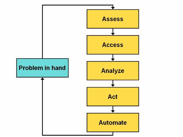
Figure 1.5-1 Life Cycle of the 5 A's Process model
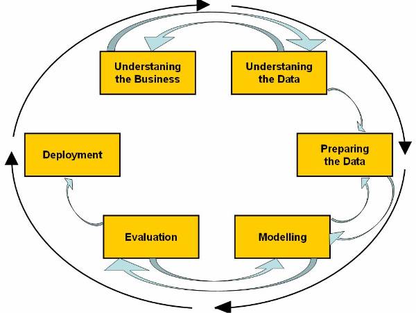
Figure 1.5-2 CRISP-DM
Cross-Industry Standard Process for Data Mining
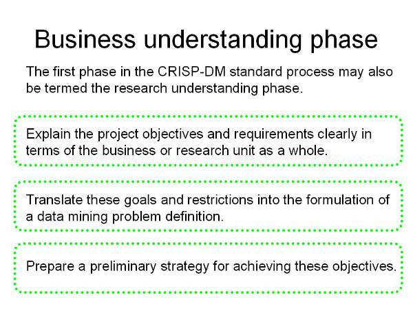
Figure 1.5-3 The CRISP-DM Process Model
Understanding the Business
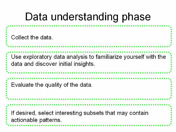
Figure 1.5-4 The CRISP-DM Process Model
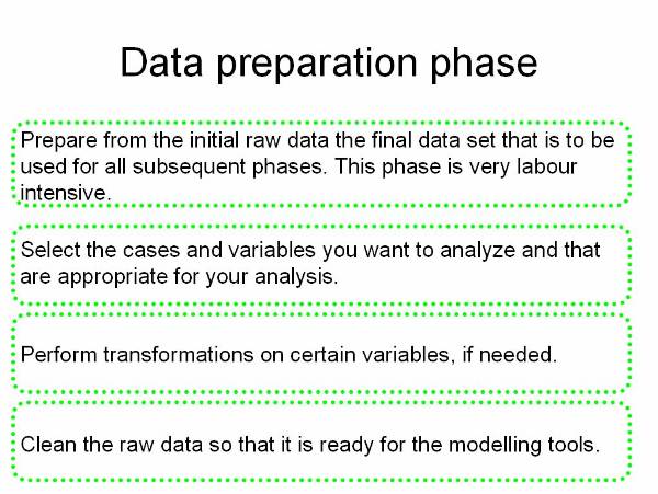
Figure 1.5-5 The CRISP-DM Process Model
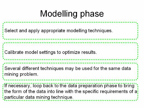
Figure 1.5-6 The CRISP-DM Process Model
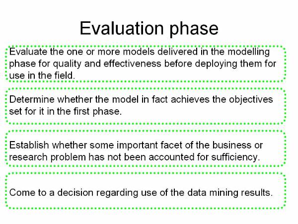
Figure 1.5-7 The CRISP-DM Process Model
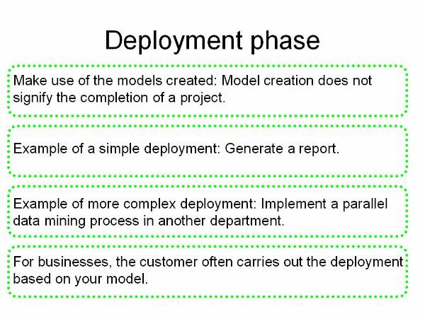
Figure 1.5-8 The CRISP-DM Process Model
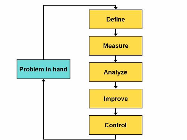
Figure 1.5-9 Life Cycle of the Six-Sigma Process Model
The 10 Commandments of Data Mining
10 Commandments or 10 Golden Rules of data
mining help the miner guide through the data preparation process: ![]()
Select clearly defined problems that will produce wanted benefits.
Specify the required solution.
Define how the solution delivered is going to be used.
Understand as much as possible about the problem and the data set.
Let the problem drive the modelling (i.e.: tool selection, data preparation).
Stipulate assumptions.
Refine the model iteratively.
Make the model as simple as possible-but not simpler.
Define instability in the model (critical areas where change in output is drastically different for small changes in inputs).
Define uncertainty in the model (critical areas and ranges in the data set where the model produces low confidence predictions/insights).
Rules 4, 5, 6, 7, and 10 have particular relevance for data preparation. Data can inform only when summarized to a specific purpose, and the purpose of data mining is to wring information out of data. Understanding the nature of the problem and the data (rule 4) is crucial. Only by understanding the desired outcome can the data be prepared to best represent features of interest that bear on the topic (rule 5). It is also crucial to expose unspoken assumption (rule 6) in case data are not warranted.
Modelling data is a process of incremental improvement (rule 7), or loosely: prepare the data, build a model, look at the results, re-prepare the data in light of what the model shows, and so on. Sometimes, re-preparation is used to eliminate problems, to explicate useful features, to reduce garbage, to simplify the model, or for other reasons. At the point that time and resources expire, the project is declared either a success or a failure, and it is on to the next one.
Uncertainty in the model (rule10) may reflect directly on the data. It may indicate a problem in some part of the data domain - lack of data, the presence of outliers or some other problem. 5 of 10 golden rules of data mining bear directly on data preparation.
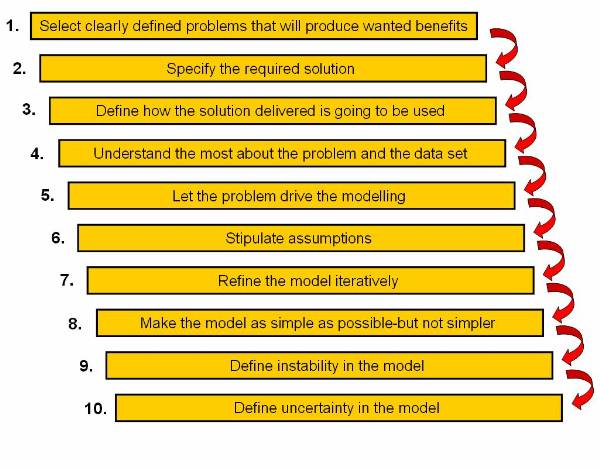
Figure 1.6-1 10 Commandments
Data Warehouse Introduction
Companies use data warehouses to store data, such as product sales statistics and employee productivity. This collection of data informs various business decisions, such as market strategies and employee performance appraisals. In today's market-scenario, a company needs to make quick and accurate decisions. The easiest way for swift retrieval of data is the data warehouse. Organizations maintain large databases that are updated by daily transactions. There databases are operational databases. These databases are designed for daily transactions and not for maintaining historical records. This purpose is solved by a data warehouse.
Objective of a Data Warehouse
Data warehouse provides the decision makers, in a company, with tools to systematically organize data and make decisions based on the data. A company maintains separate data warehouse and operational database so that the decision making body of the company functions efficiently. A data warehouse provides the decision making body of the company with a platform that provides a historical data for analysis.
You can discriminate a data warehouse from an operational database on bases of the following four concepts:
Subject-oriented: A data warehouse is designed to maintain records sales, product, supplier and customer. This is in contrast to the design of a database, which is designed to maintain daily operations. A data warehouse provides a simple and concise collection of data usually related to a particular subject that is used for decision-making in a company.
Integrated: A data warehouse is an integrated resource formed out of many other resources. These resources can be varied ranging from databases to flat files. Data from these resources is cleaned and integrated to make a consistent data warehouse.
Nonvolatile: A data warehouse has a physically separate identity and is made out of the operational data. Because of this separation, the operations on a data warehouse are restricted to updating and adding data and accessing data.
Time variant: A data warehouse is maintained by an organization for improvement and progress of the company. The decisions are made by analysing past trends in companies performance. For these decisions to be made correctly there is an explicit or implicit time constraint for each data warehouse structure.
Data Warehousing
Data warehousing is the term use to name the process of constructing and using a data warehouse. Construction of a data warehouse is done by keeping in mind that the decision making body of a company wants to get an overview of the data and not the details of the data. Construction of a data warehouse consists of three operations on data:
Data integration: Involves establishing connection between the collected data and to bring the chunks of data in a standard form.
Data cleaning: Involves removal of the data chunks, which are not useful in the decision making process.
Data consolidation: Involves combining of the data chunks and uniting them to form a data warehouse.
When a company forms a data warehouse it expects to achieve:
Customer satisfaction: A company wants to maintain a record of the customer needs. The company also maintains a record of the buying trends of its products.
Product portfolios: A company wants to manage the product portfolios so that product repositioning is possible. The decision making body refers to this data and formulate product strategies.
Profit sources: A company wants to make profits on their products. The decision making body refers to this data and finds the places where it can make profits.
Customer relationship: A company wants to maintain a homogeneous environment for its customers. The decision making body refers to this data and finds cost effective method fir customer satisfaction.
Data Warehouse Dependents
The data warehouse dependents are those parts of data warehouse, which are not directly connected with the warehouse functioning. The dependents are data repositories developed for specialized purposes. The commonly used dependents are data marts and meta-data. Data marts contain a summary of data present in the data warehouse. Meta-data is a storage place for information about data stored in data warehouse.
Data Marts
Data mart is a database that contains a subset of data present in a data warehouse. Data marts are created to structure the data in a data warehouse according to issues, such as hardware platforms and access control strategies. User can divide a data warehouse into data marts after the data warehouse has been created.
The division of a data warehouse into data marts results in faster responses to database queries, as data contained in data mart is less than data contained in a data warehouse. The two ways to implement data marting are:
Basic model of data marting
Hybrid model of data marting
The failure of data warehousing to address the
knowledge workers culture and the warehouse maintenance prompted data marting.
Data marting has two models, basic model and hybrid model. The basic model of
data marting focuses on knowledge worker needs whereas hybrid model focuses
both on business needs as well as knowledge worker needs. You can only create
data marts in basic model of data marting. Data is extracted directly to data
marts in basic model of data marting from the data sources. It is possible to
use Multi dimensional Database Management System (MDDBMS), Relation Database
Management System (RDBMS) and Big Wide Tables (BTW) to implement data marts. On
this figure is shown basic model of data marting in which data marts extracts
data from the data sources![]() . End Users access data from data
marts.
. End Users access data from data
marts.
Hybrid model of data marting has an enterprise
wide data warehouse to store data. The data inside this data warehouse is
present in both summarized and detailed form. You need to divide data warehouse
into data marts depending on needs of knowledge workers. Data sources provide
data to data warehouse. In other words data warehouse extract data from the
data sources and stores the data inside it. User can also use RDBMS, MDDBMS and
BWT to implement data marts in hybrid model of data marting to use most of the
benefits and avoids most of the limitations of both data warehouse and data
mart.![]() This Data marting hybrid model
shows how users access data stored in data marts. Data warehouse updates data
in the data marts.
This Data marting hybrid model
shows how users access data stored in data marts. Data warehouse updates data
in the data marts.
There are three approaches to implement hybrid model of data marting. The first approach is described above and remaining two approaches are:
Extracting data through data marts
Virtual data warehouse
User can use data marts in place of data
warehouse to extract data from data sources in hybrid model of data marting.
Data marts updates data warehouse with the data. Knowledge workers access the
data from the data warehouse. ![]() This figure shows a hybrid model
of data marting in which end users access data stored in data warehouse. Data
marts update data in the data warehouse.
This figure shows a hybrid model
of data marting in which end users access data stored in data warehouse. Data
marts update data in the data warehouse.
User can also use virtual data warehouse in
place of real data warehouse. The virtual data warehouse is software that
consists of data warehouse access layer. Data warehouse access layer enables
end users to access data in data marts. Data warehouse layer also controls the
data marts. ![]() This figure shows how a hybrid model of data
marting using virtual data warehouse works in an organization.
This figure shows how a hybrid model of data
marting using virtual data warehouse works in an organization.
Metadata
Metadata is information about the data in the data warehouse describing the content, quality, condition and other appropriate characteristics. In data warehouse metadata describes and defines the warehouse objects.
The metadata is stored in the metadata repository. That can be viewed as the storage place for the summary of data stored in the data warehouse. A metadata repository needs to have the following:
Structure for the data warehouse: Repository needs to contain description for the schemas of the warehouse, data hierarchies and data definitions.
Operational metadata: Repository needs to contain history if the data that are migrated from a resource and the operations performed on the data. Different stages of data are active, archived or purged. Active is current data, archived is copied data and purged is deleted data.
Summarization algorithms for metadata: Repository needs to contain measure definition algorithms and dimension definition algorithms. It should contain data on partitions, granularity and predefined queries and reports.
Mapping constructs metadata: Repository needs to contain the mapping constructs used to map the data from the operational data to the data warehouse. These include data extraction, data cleaning and data transformation rules.
System performance metadata: Repository needs to contain profiles that improve the data access and retrieval performance. It should also contain the data used for timing and scheduling of the update and deletion of data.
User can then view metadata as a summary of the data in the warehouse. There are other methods for summarizing the data in a data warehouse. These can be listed as:
Current detailed data: Maintained on disks.
Older detailed data: Maintained on temporary storage devices.
Light summarized data: Mostly temporary form of storages for backup of data and are rarely maintained on physical memory.
Highly summarized data: Mostly temporary form of storages for data transitions and are rarely maintained on physical memory as well.
Metadata is very important for a data warehouse as it can act as a quick reference for the data present in the warehouse. This acts as a soul reconstruction reference of the warehouse in case of any reconfiguration of data.
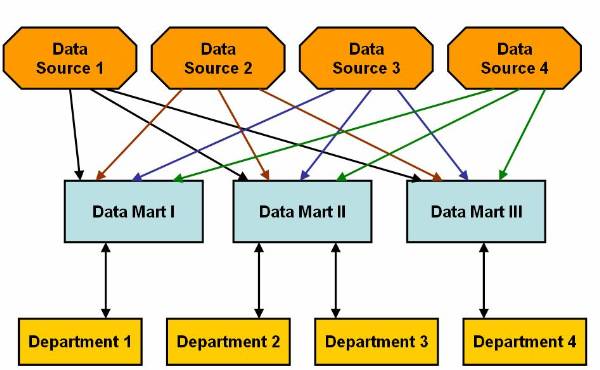
Figure 2.2-1 Basic Model of Data Marting
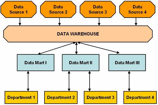
Figure 2.2-2 Hybrid Model of Data Marting
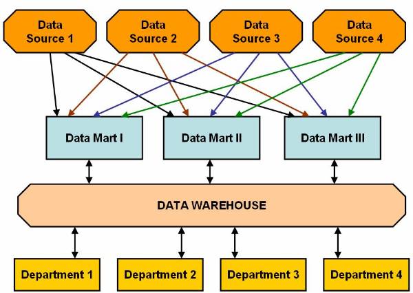
Figure 2.2-3 Extracting Data Through Data Mart
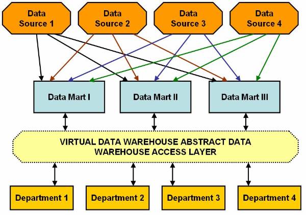
Figure 2.2-4 Virtual Data Warehouse Model of Data Marting
Data Warehouse Architecture
Data warehouse can be built in many ways. The warehouse can be based on bottom-up, top-down or even on a the combination of both of these approaches. The approach followed in designing a data warehouse determines the outcome. The data warehouse can have a layered architecture or a component-based architecture.
Process of Designing a Data warehouse
The process of warehouse design follows the approach chosen for the designing. The bottom-up approach starts with carrying experiments for organizing data and then forming prototypes for the warehouse. This approach is generally followed in early stages of business modelling and also allows testing of new technological developments before implementing them in the organization. This approach enables the organization to progress through experiments and that to at a less expense.
The top-down approach starts with designing and planning the overall warehouse. This approach is generally followed when the technology being modelled is relatively old and tested. This design process is intended to solve well-defined business problems.
The combined approach is when an organization has the benefits of a planed approach from the top-down approach and the benefits of rapid implementation from the bottom-up approach.
The constructing a data warehouse may consist of the following steps:
Planning
Requirement study
Problem analysis
Warehouse design
Data integration and testing
Development of data warehouse
Those steps can be implemented in designing a warehouse. The methods used for designing a warehouse are:
Waterfall method: Systematic and structured analysis is performed before moving to the next step of design.
Spiral method: Rapid generating of functional systems and then these are released in a short span of time.
Generally, a warehouse design process contains:
Choosing business process for modelling.
Choosing the fundamental unit of data to be represented.
Choosing the dimensions for the data representation.
Choosing various measures for fact table.
Layered Architecture of a Data Warehouse
The architecture of a data Warehouse can be
based on many approaches. One of the most commonly used approaches for
designing a warehouse is the layered architecture. It divides the warehouse
into three interrelated layers (as shown on ![]() ). The figure
). The figure ![]() shows the three-tier architecture of data
warehouse. The figure clearly discriminates the bottom tier, the middle tier
and the top tier of the warehouse design.
shows the three-tier architecture of data
warehouse. The figure clearly discriminates the bottom tier, the middle tier
and the top tier of the warehouse design.
The lowest portion of the architecture consists of operational database and other external sources for extracting data. This data is cleaned, integrated, and consolidated to form a good shape. Once this is done, the data is passed to the next stage, to the bottom tier in the architecture.
In this model of data warehouse the bottom tier is mostly a relation database system. The bottom tier extracts data from data sources and places it in the data warehouse. Application program interfaces known as gateways, such as Open Database Connectivity (ODBC) are used for the retrieval of data form data sources, such as operational databases. The gateway facilitates generation of Structured Query Language (SQL) codes for the data from the database management system. The commonly used gateways are ODBC, Open Linking and Embedding for Data Bases (OLE-DB), Java Database Connectivity (JDBC).
The middle tier of consists of OLAP servers. These servers can be implemented in the form of Relational OALP servers or in the form of Multidimensional OLAP servers. Both these approaches can be explained as:
ROLAP model is extended relational database, which maps the operations on multidimensional data to standard relation operations.
MOLAP model directly implements multidimensional data and operations.
The third tier of this architecture contains queering tools, analysis tools and data mining tools.
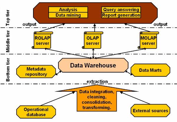
Figure 2.3-1 Architecture of a Data Warehouse
Data Warehouse Components Based Architecture
The data warehouse design based on components is
a collection of various components, such as the design component and the data
acquisition components. The design component of the data warehouse architecture
enables you to design the database for the warehouse. It collects the data from
various sources and stores it in the database of the data warehouse. ![]()
The Design Component
The design component of the data warehouse architecture enables you to design the database for the warehouse. The data warehouse designers and data warehouse administrators are design component for designing data to be stored in the database of the data warehouse. The data warehouse databases design depends on the size and the complexity of data. The designers use parallel database software and the parallel hardware in case of extremely large and complex databases. De-normalized database designs may be involved, they are known as star schemas.
The Data Manager Component
The data manager is responsible for managing and providing access to data stored in the data warehouse. The various components of data warehouse use data manager component for creating, managing, and accessing data stored in data warehouse. The managers for data can be classified into two types:
Relational Database Management System (RDBMS)
Multidimensional Database Management System (MDBMS)
The RDBMS is usually used managing data for a large enterprise data warehouse. The MDBMS is usually used for managing data for a small size departmental data warehouse. Database management systems for building data warehouse is employed according to the following criteria:
Number of users for the data warehouse
Complexities of queries give by the end user
Size of the database to be managed
Processing of the complex queries given by the end user
The Management Component
The management component of data warehouse is responsible for keeping track of the functions performed by the user queries on data. These queries are monitored and stored to keep track of the transactions for further use. The various functions of the management component are:
Manage the data acquisition operations.
Managing backup copies of data being stored in the warehouse.
Recovering lost data from the backup and placing it back in the data warehouse.
Providing security and robustness to data stored in the data warehouse.
Authorizing access to data stored in the data warehouse and providing validation feature.
Managing operations performed on data by keeping a track of alterations done on data.
Data Acquisition Component
The data acquisition component collects data from various sources and stores it in the database of the data warehouse. It uses data acquisition applications for collecting data from various sources. These applications are based on rules, which are defined and designed by the developers of the data warehouse. The rules define the sources for collecting data for the warehouse. These rules define the clean up and enhancement operations to perform on data before storing the data in the data warehouse. The operations performed during data clean up are:
Restructuring of some of the records and fields of data in warehouse
Removing the irrelevant and redundant data from that being entered in the warehouse.
Obtaining and adding missing data to complete the database and thereby make it consistent and informative.
Verifying integrity and consistency of the data to be stored.
The data enhancement operations performed on data include:
Decoding and translating the values in fields for data.
Summarizing data.
Calculating the derived values for data.
The data is store in the databases of the data warehouse after performing clean up and enhancement operations. The data is stored in the data warehouse database using Data Manipulation Languages (DML) such as SQL.
The data acquisition component creates definition for each of the data acquisition operations performed. These definitions are stored in the information directory and are known as the metadata. The various products use this metadata to acquire data from the sources and transfer it to the warehouse database. Many products can be used for data acquisition, for example:
Code Generator: Create 3 GL/4 GL capture programs according the rules defined by the data acquisition component. The code generator is used for constructing the data warehouse that requires data from large number of sources and requires extensive cleaning of the data.
Data Pump: Runs on the computer other than the data source or the target data warehouse computer, the computer running the data pump is also known as the pump server. The pump server performs data cleaning and data enhancement operations at the regular intervals and the results are sent to the data warehouse systems.
Data Replication Tool: Captures modifications in the source database at one computer and then make changes to the copy of the source database on different computers. The data replication tools are used when data is obtained from less number of the sources and requires less data cleaning.
Data Reengineering Tool: Performs data clean up and data enhancement operations. The reengineering tools make relevant changes in the structure of the data and sometimes delete the data contents such as name and the address data.
Generalized Data Acquisition Tools: Move data stored on a source computer to the target computer. The different data acquisition tools have different abilities to perform data enhancement and data clean up activities on the data.
Information Directory Component
The information directory provides details of data stored in a data warehouse. The information directory component helps the technical and the business users to know about the details of data stored in data warehouse. The information directory enables the users to view the metadata, which is the data about the data stored in the data warehouse. The metadata is prepared while designing the data warehouse and performing the data acquisition operations.
Figure ![]() shows various components of the information
directory. The main components of the information directory are the metadata
manager, metadata, and the information assistant.
shows various components of the information
directory. The main components of the information directory are the metadata
manager, metadata, and the information assistant.
The metadata manager manages the input and export metadata. The metadata stored in the information directory:
Technical data:
Information regarding the various sources of data.
Information regarding the target where the data is to be stored.
Rules to perform clean up operations on the data.
Rules to perform data enhancement.
Information regarding mapping between various sources of data and data warehouse.
Business data
Information about predefined reports and queries.
Various business terms associated with the data.
The information assistant component of the business data facilitates easy access to the technical and the business metadata. It enables to understand the data from the business point of view. It enables to create new documents, search data, analyse reports, and run queries.
Data Delivery and Middleware Component
The middle ware component provides access to the data stored in the data warehouse. The data delivery component is used for transferring data to other warehouses. The data delivery component also distributes data to the end user products such as local database and spreadsheet. The data warehouse administrator determines the data for distributing to other data warehouses. The information assistant of the information component of the data warehouse prepares the schedule for delivering data to the other warehouses.
The middleware connects the warehouse databases and end user data tools, there are two types:
Analytical Server: Assists in analysing multidimensional data.
Intelligent data warehousing middleware: Controls access to the database of the warehouse and provides the business view of the data stored in the warehouse.
Data Access Component
The data access and the middleware components provide access to the data stored in the data warehouse. The data access component consists of various tools that provide access to the data stored in a data warehouse. The various data access tools are:
Tools for analysing data, queries and reports.
Multidimensional data analysis tools for accessing MDBMS.
Multidimensional data analysis tools for accessing RDBMS.
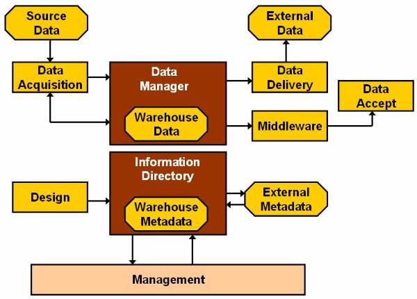
Figure 2.4-1 The Data Warehousing Architecture
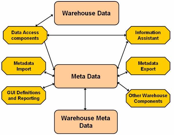
Figure 2.4-2 The Components of the Information Directory
OLAP and its Types
Large amount of data are maintained in the form of relational databases. The relational database is usually used for transaction processing. For successfully executing these transactions, the database is accompanied with highly efficient data processor for many small transactions. The new trend is to form tools that make a data warehouse out of the database.
The user needs to be able to clearly distinguish between a data warehouse and an On-Line Analytical Processing (OLAP). The first and the most prominent difference is that a data warehouse is based on relational technology. OLAP enables corporate members to gain speedy insight into data through interactive access to a variety of views of information.
Collection of data in a warehouse is typically based on two questions WHO and WHAT which provide information about the past events on the data. A collection of data in OLAP is based on questions such as WHAT IF and WHY. A collection of data is a data warehouse whereas an OLAP transforms data in a data warehouse into strategic information.
Most of the OLAP applications have three features in common:
Multidimensional views of data.
Calculation-intensive capabilities.
Time intelligence.
The Multidimensional View
The multidimensional view represents the various ways of representing data for the corporate to make quick and efficient decisions. Usually the corporate needs to view data in more than one form for making decisions. These views may be distinct of may be interlinked depending on the data represented in them. Data may consist of financial data, such as scenario of organization and time. Data may also consist of dales data, such as product sales by geography and time. A multidimensional view of data provides data for analytical processing.
The Calculation-intensive Capabilities
The calculation-intensive capabilities represent the ability of the OLAP to handle computations. The OLAP is expected to do more than just aggregating data and giving results. The OLAP is expected to do more than just aggregating data and giving results. The OLAP is expected to provide computations that are more tedious for example, calculating percentage of total records and allocation problems, which require hierarchal details.
OLAP Performance indicators use algebraic equations. These may consist of sales trend predicting algorithms, such as percentage growth. Analysing and comparing sales of a company with its competitors consists of complex calculation. OLAP is required to handle and solve these complex computations. OLAP software provides with tools for computational comparisons that enable the decision makers more self-independent.
The Time Intelligence
Any analytical application has time as an integral component. Since a business performance is always judged on time, it becomes an integral part for the decision-making. An efficient OLAP always views time as an integral part.
The time hierarchy can be used in different manner by the OLAP. For example, a decision maker can ask to see the sales for the month July or the sales for the first three months of the year 2007. The same decision maker can ask to see the sales for red t-shirts but may never bother to see the sales for the first three shirts. The OLAP system should define the period based comparisons very clearly.
The OLAP is implemented on warehouse servers and can be divided into three modelling techniques depending on the data organization:
Relational OLAP server
Multidimensional OLAP server
Hybrid OLAP server
Relational OLAP server (ROLAP)
The ROLAP server is placed between relational back-end server and client front-end tool. These servers use relational database management system for storing the warehouse data. The ROLAP servers provide optimisation routines for each database management system in the back-end. It provides for aggregation and navigation tools for the database. The ROLAP has a higher scalability than Multidimensional OLAP server (MOLAP).
Multidimensional OLAP server (MOLAP)
The MOLAP servers use array-based multidimensional storage engines for providing a multidimensional view for data. These map multidimensional views directly from data cube array structure. The advantage in using a data cube is that fast indexing and summarized data.
Hybrid OLAP server (HOLAP)
The HOLAP servers use the concepts of both MOLAP and ROLAP. This has the benefit of greater scalability as in case of the ROLAP and has faster computation power and in case of the MOLAP.
Relating Data Warehousing and Data Mining
A Data Warehouse is a place where data is stored for convenient mining. Data Mining is the process of extracting information from various databases and re-organizing to for other purposes. Online analytical mining is a technique for connecting data warehouse and data mining.
Data Warehouse Usage
Data warehouse and data marts are used in many
applications. Data in warehouses and data marts contain a refined form of data,
which is in an integrated and processed form of data and is stored under one
roof. The data maintained in data warehouse forms an integral part of the planning
closed loop structure. This figure ![]() shows the stages in decision-making process of
the organization. This process is a close loop and is completely dependent on
the data warehouse.
shows the stages in decision-making process of
the organization. This process is a close loop and is completely dependent on
the data warehouse.
The common use of data warehouse is in the following fields:
Banking services
Consumer products
Demand based production
Controlled manufacturing
Financial services
Retailer services
A data warehouse has to be fed with a large
amount of data, so that it provides information for the decision making body of
the organization. This becomes time dependent because the history of events is
an important factor in decision-making. For example, if a decision is to be
taken on changing the price of a product then for the relative change in sales,
then the decision making body needs to see data for the past years trends. The
decision-making body come to an effective conclusion making use of the data
warehouse. The data warehouse development stages figure ![]() shows that a data warehouse has three stages
in its evolution initial, progressive and final stage. In the initial stage of
evolution, a data warehouse is concerned with report generation and query
analysing. Tools used in the initial stage are database access and retrieval
tools.
shows that a data warehouse has three stages
in its evolution initial, progressive and final stage. In the initial stage of
evolution, a data warehouse is concerned with report generation and query
analysing. Tools used in the initial stage are database access and retrieval
tools.
After the initial stage the data warehouse progresses to the progressive stage. The progression is divided into two stages initial and later. In the initial part of the progressive stage, the data warehouse is used in analysing the data, which has been collected and summarized over the past period. This analysis of data is used for report generation and formulation of charts, used are database-reporting tools.
In the later part of the progressive stage, the data warehouse is used for performing multidimensional analysis and sophisticated slice and dice operation using database-analysis tools.
In the final stage, the data warehouse is employed for the knowledge discovery and making strategic decision. The decision-making body usually makes use of data mining techniques and uses data mining tools.
The data warehouse will be of no use if decision-makers are not able to use it or are not able to understand the results produces by querying the data warehouse. For this reason there are three kinds of data warehouse application:
Information-processing - this tool is intended towards supporting the data warehouse querying and it provides with these features - reporting using cross tabs, basic statistical analysis, charts, graphs or tables.
Analytical-processing - it operates on data both in summarized and detailed form and supports basic OLAP operations such as these - slice and dice, drill-down, roll-up or pivoting.
Data-mining - it provides mining results using the visualization tools and supports knowledge discovery by finding - hidden patterns, associations, constructing analytical modes, performing classification and performing predictions.
Data Warehouse to Data Mining
OLAP and data mining are disjoint, rather data mining is a step ahead from OLAP. The OLAP is data summarization and aggregation tools that help data analysis, of the other hand data mining allows automated discovery of implicit pattern and knowledge recognition in large amounts of data. The goal of OLAP tools is to simplifying and supporting interactive data analysis, whereas the goal of data mining tools is to automate as many processes as possible.
Data mining can be viewed in the form where it covers both data description and data modelling. The OLAP results are directly based on summary of data present in data warehouse. This is useful for summary based comparison. This is also provided by data mining but is an inefficient or an incomplete utilization of the capabilities of data mining. Data mining is capable of processing data at much deeper granularity levels than just processing data, which is stored in data warehouse and it has the capability of analysing data in transactional, spatial, textual and multimedia form.
On-Line Analytical Mining (OLAM)
There is a substantial amount of research carried out in the field of data mining in accordance with the platform to be used. The various platforms with which data mining has been tested are:
Transaction databases
Time-series databases
Relational databases
Spatial databases
Flat files
Data warehouses
There are many more of the platforms with which data mining has been successfully tested. One of the most important is integration of On-Line Analytical Mining, also known as OLAP mining. This facilitates data mining and mining knowledge in multidimensional database, which is important for the following four reasons:
High Quality of data in data warehouse
Information processing structure surrounding data warehouse
OLAP based exploratory data analysis
On-line selection of data mining functions.
An OLAM server performs similar
operations as that of the OLAP server, as it is shown on ![]() , where OLAM and OLAP servers are
together.
, where OLAM and OLAP servers are
together.
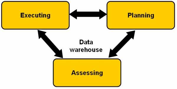
Figure 2.6-1 Closed
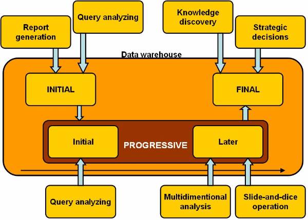
Figure 2.6-2 Data Warehouse Development Stages
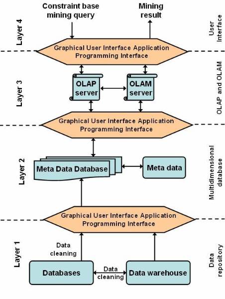
Figure 2.6-3 OLAM and OLAP Servers Together
Introduction to Classification
Classification is one of the most simple and highly used techniques of data mining. In classification data needs to be divided into segments and then make distinct non-overlapping groups. For dividing data into groups user has to have certain information about the data. This knowledge about data is most important for performing any type of classification.
Classification problems aim to identify the characteristics that indicate the group to which each case belongs. This pattern can be used both to understand the existing data and to predict how new instances will behave. Data mining creates classification models by examining already classified data (cases) and inductively finding a predictive pattern. Sometimes an expert classifies a sample of the database, and this classification is then used to create the model which will be applied to the entire database.
In the preceding definition, classification is displayed as mapping from the database to the set of classes. The classification process is divided into two phases:
Developing a model for evaluating and training data.
Classifying tuples from target database.
The basic methods that can be used for classification are:
Specifying boundaries: Provides a method for classification by dividing input database into categories. Each of these categories is associated with a class.
Probability distribution: Determines the probability definition of a class at a particular point. Consider a class Cj, the probability definition at one point ti is P (ti | Cj). In the definition, each tuple, is considered to have a single value and not multiple values. If the probability of the class is known to be as P (Cj), then the probability that ti is in the class Cj is determined by the equation: P (Cj) = P (ti | Cj)
Using posterior probability: Determines the probability for each class. The posterior probability for each class is computed and tj is assigned to the class with highest probability. For example for a data value ti, the probability that ti is in the class Cj can be determined. The equation for posterior probability is: P (Cj / ti)
Consider a database based on the values of the
two variables such that the tuple t = [ x, y ] where 0 £ x £ 10 and 0 £ y £ 12. Display the values of x and y
on graph. Figure ![]() shows the points plotted in graph. The
following figure
shows the points plotted in graph. The
following figure ![]() shows, that the reference classes dividing the
whole reference space into three classes A, B, and C. And this figure
shows, that the reference classes dividing the
whole reference space into three classes A, B, and C. And this figure ![]() shows the data in the database classified into
three classes.
shows the data in the database classified into
three classes.
Example:
User can categorize the weight of different
people and classify them into categories. Table 4 ![]() lists the attributes of database. The output
of the table can be categorised in two categories. In the first category, user
is concerned about the gender of the person. The rules for the output
classification are:
lists the attributes of database. The output
of the table can be categorised in two categories. In the first category, user
is concerned about the gender of the person. The rules for the output
classification are:
65 < weight over weight
£ weight £ normal
weight < 50 under weight
The output of the second category is based on the output of the first category. The gender of person has to be considered in second category, and here are the rules:
male
70 < weight over weight
£ weight £ normal
weight < 55 under weight
female
55 < weight over weight
£ weight £ normal
weight < 45 under weight
The classification mentioned in the second output is not as simple as the first output, as in the second output there are used classification techniques based on many complex methods.
Methods of classification which can be chosen
from based on algorithms ![]()
Statistics based algorithms
Distance based algorithms
Decision tree based algorithms
Neural network based algorithms
Rule based algorithms
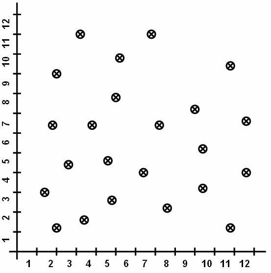
Figure 3.1-1 Data in Database
Graph with the plotted points
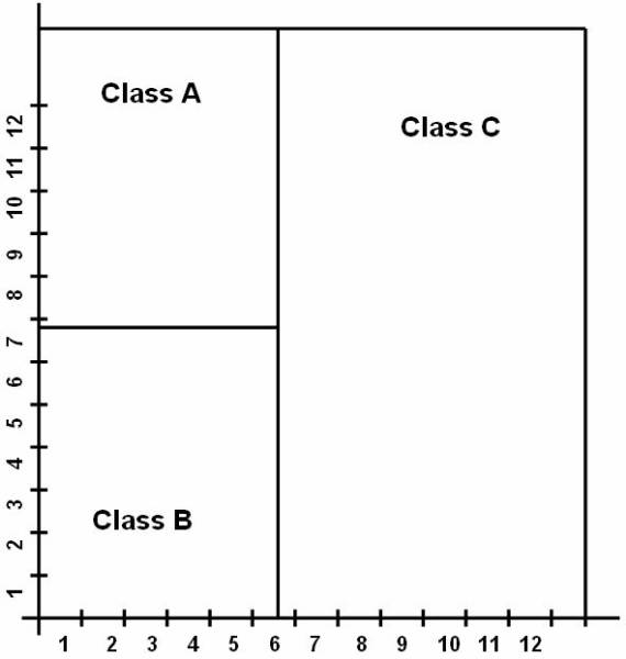
Figure 3.1-2 Reference Classes
Distribution of the classes for the classification purpose.
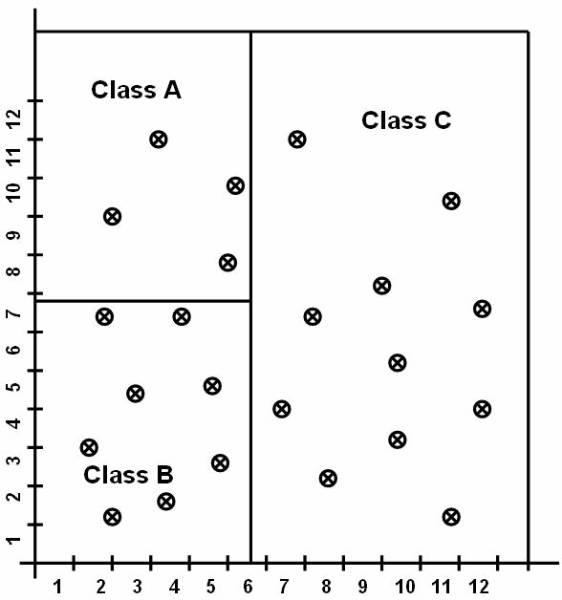
Figure 3.1-3 Data Items Placed in Different Classes
The data in the database are classified into three classes.
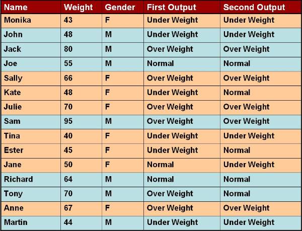
Figure 3.1-4 Database Attributes
List of the attributes of database.
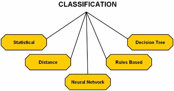
Figure 3.1-5 The Classification Methods as Applied to Data
The Distance Based Algorithms
In the Distance Based algorithm, the item mapped to a particular class is considered similar to the items already present in that class and different from the items present in other classes. If the above statement is true then the alikeness or similarity is used to measure the distance between items. This distance is termed as alikeness that is the measure of difference between the items. The concept of similarity is same as the one used in string matching or that followed by the search engines over the Internet. The databases in this search process are the Web pages. In case of search engines over the Internet, the Web pages are divided into two classes:
Those that answer the search query given to the search engine.
Those that do not answer the search query given to the search engine.
This proves that those Web pages that answer users query are more alike to query than those that did not match. The pages retrieved by the search engine are similar in context, all containing the same set of keywords in the user search query.
The concept of similarity is applied to more general classification methods. The user needs to decide the similarity check criteria and after those are decided, they are applied to the database. Most of the similarity checks depend on discreet numerical values so these are not applied to databases with abstract data types.
There are two approaches followed for classification on the bases of distance:
Simple approach
K nearest neighbors
Simple Approach
For understanding the simple approach is important that user know about the information retrieval approach, where information is retrieved from the textual data. The development of the information helps the user retrieve the data from the libraries. The basic request for data retrieval will be finding all library documents related to a particular query because in order to generate a result there needs to be some kind of comparison for query matching.
Information Retrieval System
The information retrieval system consists of libraries, which are stored in a set of document, which can be represented as:
D =
The input given as a query for search purpose consists of keywords, for example the query string can be denote with 'q'. The similarity between each document present in the document set and the query given is calculated as:
Similarity ( q, Di )
This similarity function is a set membership function, and it describes similarity between the documents and the query string given by the user. Measuring the performance of the information retrieval process is done by two methods: Precision and Recall.
The precision equation answers the question: Are the documents retrieved by matching of the information retrieval process, are those required by me and will they give me the required information? The precision equation can be display as:
This recall equation answers the question: Does the matching process of information retrieval process retrieve all documents matching the query?

This figure ![]() shows the working of the query processing. And
the following figure
shows the working of the query processing. And
the following figure ![]() displays the four possible results generated
by the information retrieval querying process.
displays the four possible results generated
by the information retrieval querying process.
User can use an equation for clustering the output. The equation to cluster the output is:
Similarity ( qi, Dj)
The concept of inverse document frequency result is used for similarity measure purposes. For example, for a given relation equation there are n number of documents to be searched, k is the keywords in the query string, and I signifies the inverse document frequency. The equation to represent the inverse document frequency result is:
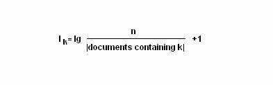
The information retrieval process enables the user to associate each distinct class to a shortcut, which represents the class. For example, the function to represent a tuples ti as a vector is:
ti = <ti1, ti2, ti3, , tik>
The functions to define a class using vector of tuples is:
Cj = <CJ1, Cj2, Cj3, , Cjk>
The user can define the classification problem as a tuples database D = , where ti = <ti1, ti2, ti3, , tik> and a set of classes C = , where Cj = <Cj1, Cj2, Cj3, , Cjk> , the classification problem is to assign each ti to class Cj such that for each Ci ¹ Cj.
User need to calculate the respective representative for each class to calculate the similarity measures. The equation to calculate the similarity measure is:
similarity (ti, Cj) similarity (ti, C1) ; C1IC
The
following figure ![]() shows the representation of each class for
classification purpose and it shows the classes with their respective
representative point.
shows the representation of each class for
classification purpose and it shows the classes with their respective
representative point.
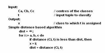
Algorithm follows the distance-based approach for assuming that for each class is represented by its center. For example the user can represent the centre of Class A as Ca, the centre of Class B as Cb, and centre of Class C as Cc. To perform simple classification the user have the following pseudo code:
The K Nearest Neighbors
The K nearest neighbor is the most commonly used method for finding the distance measures. This technique is based on the assumption that the database contains not only data but also the classification for each item present in the database.
This
approach works as if a new item is to be added and classification is to be made
for this item. Instead of calculating its distance from all the other items in the
K nearest neighbor approach the distance with the K closest items is calculated
for each class. The new item is placed in the class, which has the highest
density for the K closest items. This figure ![]() shows the training points as K=4.
shows the training points as K=4.
The pseudo code to perform K nearest neighbor classification is:
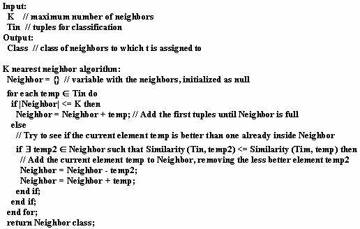
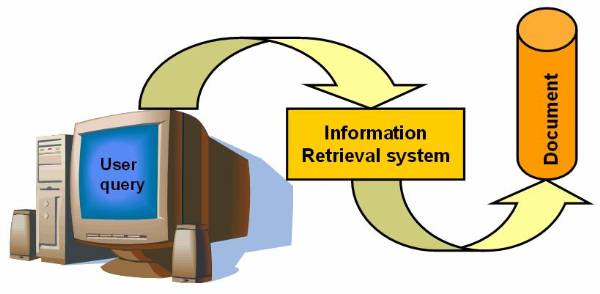
Figure 3.2-1 Working of the Query Processing
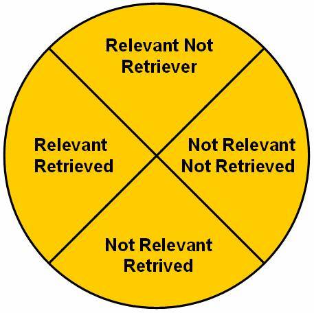
Figure 3.2-2 Four Possibilities of the Querying Process
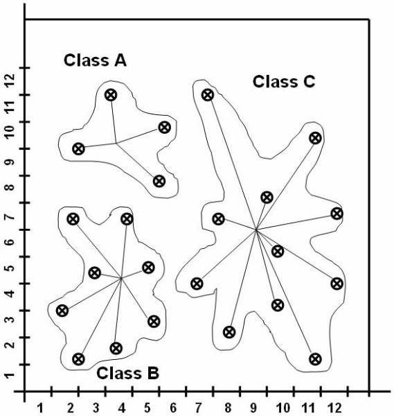
Figure 3.2-3 Representation of Classes for Classification
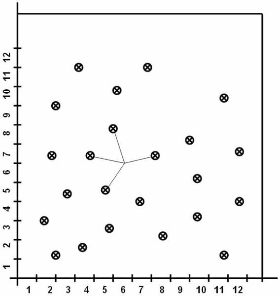
Figure 3.2-4 Training Points
Training points as K=4.
The Decision Tree Based Algorithms
Decision tree method for classification is based on construction of a tree to model classification process. When the complete tree is constructed it is applied to each tuple and hence does classification for each, and there are two steps involved:
Building the tree named as decision tree.
Applying the decision tree to database.
In this approach classification is performed by dividing the search space into sections, these are rectangular regions. The tuple is classified on the basis of the region it is placed in. User can define a decision tree as:
A tuple database D= , where ti = <ti1, ti2, ti3, , tik>, and that the database schema contains the attribute as a set A = and the class is denoted by the set C= , where Cj = <Cj1, Cj2, Cj3, , Cjk>
Decision tree is a tree associated with D as it has the following properties:
Each node is labelled with a predefined attribute Ai
Each leaf node is labelled with a class Cj
Each arc is labelled with a predicate that can be applied to the attribute associated with parent.
The decision tree consists of two parts
Induction constructs a decision tree for the data in the database or training data.
For each tuple ti I D apply the decision tree, as this will determine its class.
This decision tree ![]() represents the logic for mapping.
represents the logic for mapping.
The pseudo code to represent the decision tree method is:
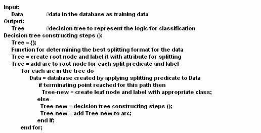
In
the above pseudo code, splitting attributes are used to label the nodes. The
splitting predicates are represented by arcs. The splitting predicates for
gender are male and for the weight
are . The
training data can be formulated in different ways as shown on following
figures. Figure ![]() shows the decision tree.
shows the decision tree.
The
balanced tree ![]() is a type of decision tree used to analyse the
data present in the database. The rectangular splitting of database region is
also done according to the balanced tree. The tree has the same depth irrespective
of the path taken to reach from the root node to a leaf node.
is a type of decision tree used to analyse the
data present in the database. The rectangular splitting of database region is
also done according to the balanced tree. The tree has the same depth irrespective
of the path taken to reach from the root node to a leaf node.
A
deep tree is used for classifying training data. Figure ![]() shows the decision tree, which is used for the
weight classification. The rectangular splitting
shows the decision tree, which is used for the
weight classification. The rectangular splitting ![]() of database region is also done according to
the deep tree.
of database region is also done according to
the deep tree.
A
Bushy tree is type of decision tree used for classifying training data as shows
figure ![]() . It is not a balanced tree that is
the depth for all leafs is not equal. The rectangular splitting
. It is not a balanced tree that is
the depth for all leafs is not equal. The rectangular splitting ![]() of database region is also done according to
the Bushy tree.
of database region is also done according to
the Bushy tree.
The
training data can be also classified through a decision tree, known as
incomplete decision tree ![]() . The incomplete decision tree is not
having a clause for gender. This figure
. The incomplete decision tree is not
having a clause for gender. This figure ![]() shows rectangular splitting of the database space
based on the incomplete decision tree.
shows rectangular splitting of the database space
based on the incomplete decision tree.
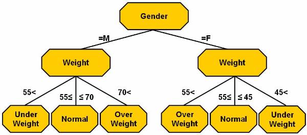
Figure 3.3-1 The Decision Tree
Decision tree for the table from 'Introduction to Classification
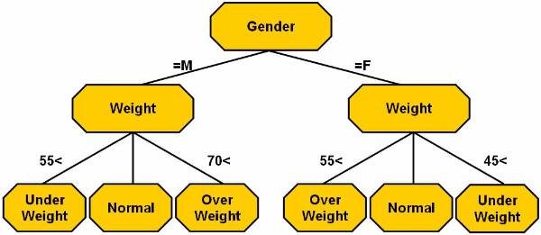
Figure 3.3-2 The Decision Tree
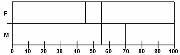
Figure 3.3-3 Rectangular Splitting of a Balanced Tree
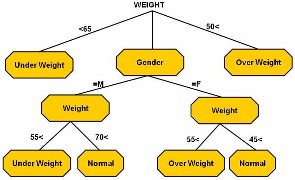
Figure 3.3-4 Decision Tree Used for Weight Classification
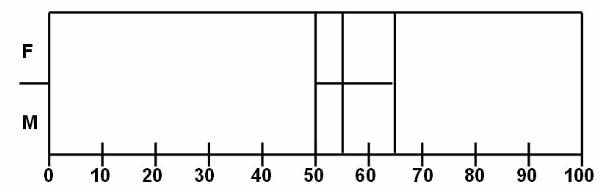
Figure 3.3-5 Rectangular Splitting for Deep Tree
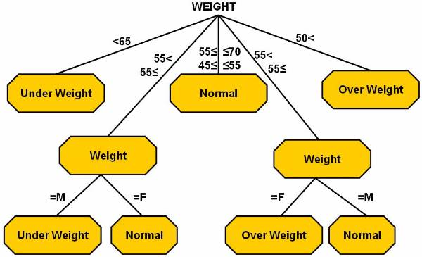
Figure 3.3-6 The Bushy Tree
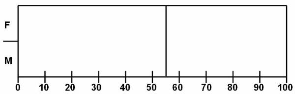
Figure 3.3-7 Rectangle Splitting
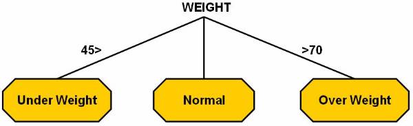
Figure 3.3-8 Incomplete Decision Tree
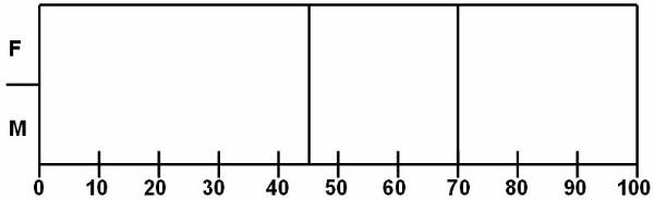
Figure 3.3-9 Rectangular Split for Incomplete Decision Tree
The Neural Network Based Algorithms
In neural network, a model is created which gives a format of representing data. When a tuple is classified, values of attributes related to the tuple are redirected into a graph. This input is given at the corresponding source node. In neural network method there is a sink node for each class. The output generated predicts that whether the tuple added belongs to the class or not. The tuple is assigned according to the output generated by each class.
The classification of neural network involves the learning process which is termed as the filtering of the tuple through the starting structure. User can solve a classification problem using neural networks as:
Determine the number of output nodes and attributes to be used as input.
Determine the labels and functions to be used for the graph
Determine the functions for the graph.
Each tuple needs to be evaluated by filtering it through the structure or the network.
For each tuples ti I D, propagate ti through the network and classify the tuple.
When we classify the database items using neural network, there are many issues involved which are:
Deciding the attributes to be used as splitting attributes.
Determination of the number of hidden nodes.
Determination of the number of hidden layers to choose the best number of hidden nodes per hidden layer.
Determination of the number of sinks.
Interconnectivity of all the nodes.
Using different activation function
Propagation in Neural Network
Propagation is used for filtering and processing data in the neural network approach of classification. Output of each node i is in neural network is based on the definition of a function fi, which is called activation function. Consider an activation function fi, when applied to an input and weights , the sum if these input is:
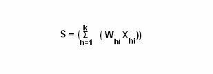
Considering that the input tuples is X where Xi = <Xi1, Xi2, Xi3, , Xik> and the output tuples is Y where Yi=<Yi1, Yi2, Yi3, , Yik>
Radial Basis Function Networks
A function, which changes its value as it moves closer to or away from central point is known as a radial function. The radial function is also called as radial basis function. It can be displayed using the Gaussian as:
Fi (S) = e (-S2/V)
Assume the input to be X1, X2,
X3, , Xk , the function be f1, f2,
f3, , fk and the output to be a summation of Y1,
Y2, Y3, , Yk and collectivity termed as Y.
This figure ![]() shows the basic structure for a Radial based
function which has only one output.
shows the basic structure for a Radial based
function which has only one output.
Perceptron
The neural network of the simplest type is
perceptron. The perception is a sigmoidal function that is a summation
function. This figure ![]() shows the perceptron classification and shows
the input being transformed into the output. It is used to classify and divide
into two different classes.
shows the perceptron classification and shows
the input being transformed into the output. It is used to classify and divide
into two different classes.
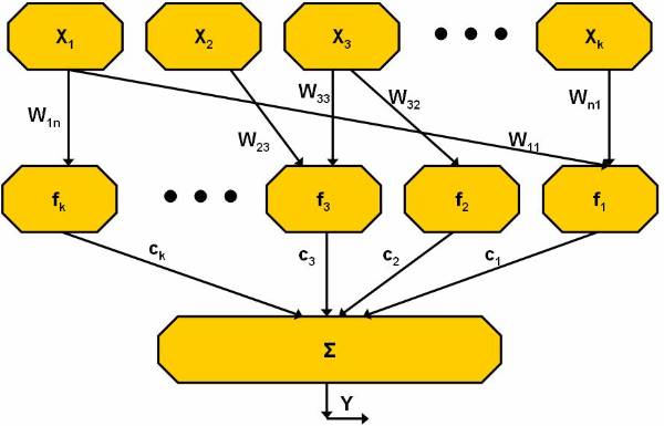
Figure 3.4-1 Radial Based Function Network
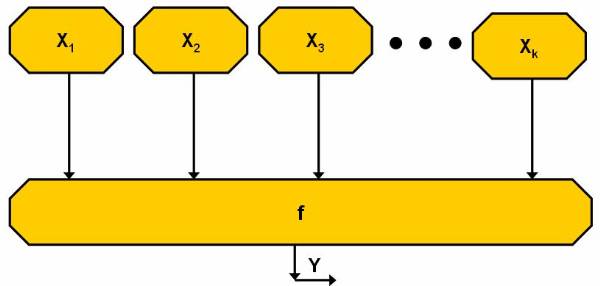
Figure 3.4-2 Classification by Perceptron
The Rule Based Algorithms
The concept of classification is for generating rules about the data and the classification is intended towards the generation of 'if then else' rules for classification. This table shows the difference between the decision tree and the rules:
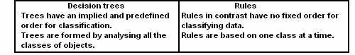
Generating Rules from a Decision Tree
It is possible to generate rules for a decision tree using the pseudo code:
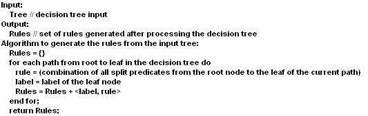
Generating Rules by Covering Method
Deriving classification rules from a neural network increases the feasibility and understanding of the neural network. Problem with generation of rules is that there are no explicit demarcation for the rules in the neural network structure. Basic idea of the pseudo code is to cluster the output with hidden nodes and input. Following is the pseudo code for the generating rules from the neural network:
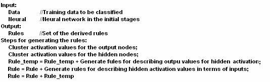
Generating Rules by Covering Method
In the covering method of rules generation does not use the decision trees neither it uses the neural network method for rules generation. In the tree, the method of rule formulation has a top down approach where rules are generated for covering a certain class as shown on this pseudo code for classifying:
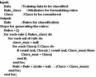
Introduction to Cluster Analysis
A cluster is a collection of data objects that have similarity with objects within the same cluster and dissimilarity with the objects of other clusters. A cluster analysis is the process of analysing the various clusters to organize the different objects into meaningful and descriptive objects. Cluster analysis is used in many applications such as data analysis, image processing, market research or pattern recognitions. By clustering user can identify dense and sparse regions and discover overall distribution patterns and interesting correlations among data attributes. The various fields, where clustering techniques can be used are:
biology - to develop new plants and animal taxonomies.
business - to enable marketers to develop new distinct groups of their customers and characterize the customer group on basis of their purchasing
identification of groups of automobiles insurance policy consumer
identification of groups of house in a city on the basis of house type, their cost and geographical location
Web - to classify the document on the Web for information discovery
Requirements of Cluster Analysis
The basic requirements of cluster analysis are:
Dealing with Different Types of Attributes: Many clustering algorithms are developed to cluster interval-based (numerical) data, while many applications require other types of data such s binary data, nominal data, ordinal data or mixture of these data types.
Dealing with Noisy Data: Generally a database consists of outliers, missing, unknown or erroneous data, but many clustering algorithms are sensitive to such type of noisy data.
Constraints on Clustering: Many applications need to perform clustering under various constraints. User wanting to search the location of a person in a city on the Internet uses the cluster households considering the constraints such as the street, area or house number for city.
Dealing with Arbitrary Shape: Many clustering algorithms
determine the clusters using Euclidean or
High Dimensionality: A database or data warehouse consists of various dimensions and attributes. Some clustering algorithms are well working with low-dimensional data that contains two or three-dimensional data, for those high-dimensional data new algorithms is required.
Input Data Ordering: Some clustering algorithms are sensitive to the order of input data. For example, the same set of data is input with different ordering, which can cause some error.
Interpretability and Usability: The result of the clustering algorithms should be interpretable, comprehensible and usable.
Determining Input Parameter: Many clustering algorithms require and user to input some parameter on cluster analysis at run time. The clustering results are sensitive to the input parameter. Parameters are very hard to determine for high-dimensional objects.
Scalability: Many clustering algorithms work well on small data sets that consist of fewer than 250 data objects. While a large database consists of millions of objects, highly scalable clustering technique is needed.
For cluster analysing, user has to study various types of data such as interval-scaled, binary or nominal and clustering methods such as partitioning method, hierarchical method, or density-based methods.
Types of Data
There are several types of data that are used in cluster analysis. User needs to know how to pre-process these data for cluster analysis. For example, a database consists of n number of objects, where each object represents person, house, company, city, or country. There are two types of data structures that are used in main memory-based clustering algorithms:
Data Matrix: It is a relational table of n x p matrix, where n = objects and p = variables. Data matrix is also called as object-by-variable structure. For example, a data set of n objects represents automobiles with p variables such as model number, model name, weight, dimension, or colour. The representation of n x p matrix is:
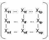
Dissimilarity Matrix: It is represented in the form of a relational table of n x n matrix, where n represents the objects. The n x n matrix is:
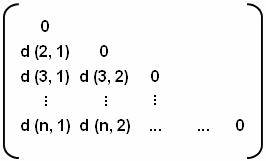
In this matrix, d (i, j) is the dissimilarity between objects i and j. The value of d (i, j) is always positive number and if the value of i and j are the same, the value of d (i, j) becomes 0. The dissimilarity d (i, j) can be calculated by various types of variables such as interval-scaled variables, binary variables, nominal variables or mixed variables.
Interval-Scaled Variables
Interval-scaled variables are continuous
measurements of linear scale. For example, height and weight, weather
temperature, or coordinates for any cluster. You can calculate these
measurements using Euclidean distance,
Calculating the mean absolute deviation, Sf using this formula:
Sf = 1/n (|X1f + Mf| + |X2f + Mf| + + |Xnf-Mf|)
Where, X1f Xnf are n measurements of f and Mf is the mean value of f that is equal to the simple mean:
Mf = (X1f + X2f + + Xnf) / n
Calculate the standardized measurement using the formula:
Zif = (Xif - Mf) / Sf
Where Zf is known as the standardized measurement. Once Z-score is calculated, dissimilarity between objects can be computed using one of these distance techniques:
Euclidean Distance: It is simply the geometric distance between multidimensional spaces. The dissimilarity between the objects is computed as:
d (i, j) =
where i = (Xi1 + Xi2 + + Xin) and j = (Xj1 + Xj2 + + Xjn) are two n-dimensional data objects.
Manhattan Distance: It is simply the average
difference of the various dimension objects. The distance measured by this
distance is same to the Euclidean distance. The dissimilarity between objects
are computed as:
d (i, j) = Σn |Xi - Xj|
where i = (Xi1 + Xi2 + + Xin) and j = (Xj1 + Xj2 + + Xjn) are also two n-dimensional data objects.
Minkowski Distance: It is generalization of both Euclidean distance and Manhattan distance. Sometime one object wants to increase or decrease the progressive weight. The dissimilarity between objects is computed as:
d (i, j) = 1/q
where i = (Xi1 + Xi2 + + Xin) and j = (Xj1 + Xj2 + + Xjn) are also two n-dimensional data objects and q is a positive integer. When the value of q is equal to 1, it represents the Manhattan distance and when q = 2, it represents the Euclidean distance.
Binary Variables
Binary variables are understood by two states 0 and1, when state is 0, variable is absent and when state is 1, variable is present. For example, an object 'employee' has a variable tax that has two states, 1 shows that the employee pays the tax and 0 shows that the employee does not pay the tax. There are two types of binary variables, symmetric and asymmetric binary variables. Symmetric variables are those variables that have same state values and weights, while asymmetric variables are those variables that have not same state values. There are two steps to calculate the dissimilarity between objects that are describing either symmetric or asymmetric binary variables.
A sample of a dissimilarity matrix of the given binary data is computed, for example, a 2 x 2 contingency table that holds all the same weight binary variables:
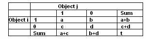
The number of the variables is equal to 1 for both the objects i and j, b is the number of variables, which is equal to 1 for object i and 0 for object j, c is the number of variables, which is equal to 1 for objects j and 0 for object i and d is the number of the variables, which is equal to 0 for both the objects i and j. So the total number of variable t = (a + b + c + d).
To calculate the dissimilarity between the objects is usually used either simple matching coefficient of jacquard coefficient. When calculating the dissimilarity between the objects that are describing symmetric binary variables, simple matching coefficient is used and when calculating the dissimilarity between the objects that are describing asymmetric binary variables, jacquard coefficient is used. The dissimilarity between objects using simple matching coefficient is:
d (i, j) = (b + c) / (a + b + c + d)
and dissimilarity between objects using jacquard coefficient is:
d (i, j) = (b + c) / (a + b + c)
For example, a company record table contains the name of the employee, gender, graduate, tax payee, experience, mobile, car and home. Name represents the object, gender is a symmetric variable and remaining variables are asymmetric variables. If employee is graduate, tax payee, has experience, has mobile, has cal, has house, then the value Y is set to 1 and the value N is set to 0. Relational table that contains binary variables:
The distance between each pair of three employees in a company can be calculated using Jacquard coefficient.
d (i, j) = (b + c) / (a +b +c)
For dissimilarity between Joe and Ross, values of a = 2, b = 2, c = 1.
d (Joe, Ross) = (2 + 1) / (2 + 2 + 1) = 0.6
For dissimilarity between Joe and Jane, values of a = 1, b = 3, c = 2.
d (Joe, Jane) = (3 + 2) / (1 + 3 + 2) = 0.84
For dissimilarity between Ross and Jane, values of a = 2, b = 1, c = 1.
d (Ross, Jane)= (1 + 1) / (2 + 1 + 1) = 0.5
These all measurements shows, that Joe and Jane have maximum dissimilarity while Ross and Jane have maximum similarity among three employees.
Nominal, Ordinal, Ratio-Scaled Variables
A nominal variable is a generalization of the binary variable and has more than two states. For example, a nominal variable, colour consists of four states, red, green, yellow, or black. In nominal variable, the total number of states is equal to N that is denoted by letters, symbols, or integers. The dissimilarity between two objects, such as i and j is calculated by using simple matching approach, which is:
d (i, j) = (t - m) / t
where m is the number of matches and t is the total number of variables.
An ordinal variable also has more than two states but all these states are ordered in a meaningful sequence. For example, in sports, gold, silver and bronze have a meaningful sequence. The gold is for first position silver is for second position and bronze for third position. The dissimilarity between the n objects that describes a set of ordinal variable sis computed by following steps, where f is a variable that is taken form set of ordinal variables:
If value of f for the ith object is Xif and f has Mf ordered states, represents the ranking 1 Mf. Replace each Xif by its corresponding rant Rif I 1 Mf
Each ordinal variable has a different number of states. So there is need to equalize the weight of all the ordinal variable. It can be done by replacing the rand Rif of the ith object in the fth variable by:
Zif = (Rif - 1) / (Mf - 1)
Dissimilarity can be computed by any of the distance measure approaches such as Euclidean distance, or Manhattan distance using Zif that represents the f value for the ith object.
A ratio-scaled variable makes positive measurements on a non-linear scale, such as exponential scale, using the formula:
AeBt or Ae-Bt
where A and B are positive constants. The dissimilarity between objects that describes the ratio-scaled variables is computed by follow with three methods:
Use Ratio-scale variable as interval-scaled variables. It is not the suitable method for calculating the dissimilar distance because in this method, the scale may be distorted.
Apply logarithmic transformation to a ratio-scale using the formula: Yif = log (Xif), where Xif is the value of variable f for object i and Yif is used as interval-valued variable.
Use the Xif as continuous ordinal data and rank (Rif) is used as interval-valued variable.
Mixed Variables
For computing the dissimilarity between the objects that describes mixed variables two following approaches are used:
Grouping all the same types of variables in a particular cluster and performing separate dissimilarity computing method for each variable type cluster. This is simple and widely used in the applications.
Grouping all the variables of different types into a single cluster using dissimilarity matrix. While making a set of common scale variables and the common scale set consists of p mixed types of variables, the dissimilarity between the objects i and j is:
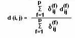
where, if either Xif or Xjf is missing, or Xif = Xjf =0 and variable f is asymmetric variable, then the indicator is
![]()
otherwise,
![]()
The contribution of variable f to the dissimilarity between objects i and j depends upon the variable types. If f is binary or nominal, then
![]()
otherwise,
![]()
If the f is interval-scaled variable, then
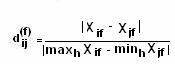
and where h is used in non-missing objects for variable f. If f is ordinal or ratio-scale variable, then first rank (Rif) is compute and Zif calculated:
Zif = (Rif - 1) / (Mf - 1)
Now this Zif is used as interval-scaled variable.
Partitioning Method
In partitioning method, a partitioning algorithm arranges all the objects into various partitions, where total number of partitions is less than the total number of objects. For example, a database of n objects can be arranged into k partitions, where k < n, where each partition represents a cluster. The partitioning depends upon a similarity function which is criteria based and clusters are formed upon it. For example, similarity function can be used to measure distance between objects, and are similar in the cluster. The two types of partitioning algorithms are k-means and k-medoids.
The K-means Method
The K-means algorithm partitions all the n objects into k clusters, so that each cluster has maximum intra-cluster similarity and minimum inter-cluster similarity. Cluster similarity is measured by the centre of gravity of a cluster. The k-means algorithm works on following steps.
Select k objects randomly that represents a cluster mean or centre of gravity of a cluster.
Assign an object to the cluster for which cluster mean is most similar based on dissimilar distance.
Update cluster mean of each cluster, if necessary.
Repeat this process until the criterion function converges all the clusters.
The K-mean algorithm takes n objects and number of cluster k as its input and returns the k cluster that minimize the squared-error criterion, which is defined as:
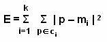
Where E si the sum of square-error for all n objects, p represents and object that is given object and mi represents the mean of the Ci cluster.
For example, a database that
containing 20 objects and user wants to arrange into 4 clusters. According to
k-mean algorithm, first random selection of 4 objects as the cluster centre.
Remaining objects are distributed to a cluster on the basis of cluster centre
to which the object is similar. This distribution is enclosed by the dotted
curves. This figure ![]() shows the 4 objects by X sign that
represents the cluster centre. Remaining objects are distributed among these
objects.
shows the 4 objects by X sign that
represents the cluster centre. Remaining objects are distributed among these
objects.
Now recalculate the mean of the
clusters based on the objects that are presented in a cluster and redistribute
the objects on basis of new cluster centre. This redistribution is also
enclosed by the dotted curves. This figure ![]() shows the redistribution of the objects on the
basis of the similarity of the centre cluster to other objects.
shows the redistribution of the objects on the
basis of the similarity of the centre cluster to other objects.
The re-clustering process is
continued until redistribution is finished and the redistributing process
returns the desired clusters. The resulting clusters are enclosed by solid
curves. This figure ![]() shows the final clusters that are returned by
the k-mean algorithms. After this, process is terminated.
shows the final clusters that are returned by
the k-mean algorithms. After this, process is terminated.
The K-medoids Method
The K-means algorithm does not work properly with large value objects. In k-medoids method, reference point is used, known as medoids instead of centre cluster. The partitioning is based on the sum of the dissimilarities between each object and its reference point (medoids). Consider a database, which consists of n objects and you want to partition these objects into k clusters. Oi is considered as a random medoids and Orandom as random object that is compared with the medoid. The K-medoids algorithm works on following steps:
Randomly select k objects that represent a reference point, medoid.
Assign remaining object to a cluster that is most similar to its medoid.
Randomly select a non-medoid object Orandom.
Calculate the total cost C of swapping the medoid Oi with non-medoids object Orandom by cost function that is used to determine the dissimilarity between Orandom and Oi.
Swap medoid Oi with the non-medoids object Orandom to make new medoids, if total cost of swapping is negative.
Process it again starting from step 2 and this process is repeated until no swapping occurs.
The e-medoids algorithm takes n objects and k number of clusters as input and produces a set of k clusters s output. For example, a database which consists n objects. Oi is a current medoid, Oj is another object and Orandom is a n neural network n-medoid object, where P is a sample object that belongs to Oi or Oj and i is not equal to j. To check, whether the swapping is possible or not, there are four cases:
P is currently assigned to Oi
and P is closer to Oj. If Oi is
swapped by Orandom, then P is reassighed to Oj.
Figure ![]() shows the reassignment of sample object P
from current medoid Oi to new medoid Oj. In
this figure single-line shows the location before swapping and double-line
shows the location after swapping.
shows the reassignment of sample object P
from current medoid Oi to new medoid Oj. In
this figure single-line shows the location before swapping and double-line
shows the location after swapping.
P is currently assigned to Oi
and P is closer to Orandom. If Oi is
swapped by Orandom then P is reassigned to Orandom.
This figure ![]() shows the reassignment of sample object P
from current medoid Oi to new medoid Orandom.
In this figure single-line shows the location before swapping and double-line
shows the location after swapping.
shows the reassignment of sample object P
from current medoid Oi to new medoid Orandom.
In this figure single-line shows the location before swapping and double-line
shows the location after swapping.
P is currently assigned to Oj
and P is closer to Oj. If Oi is
swapped by Orandom, then position of P remains
unchanged. This figure ![]() shows that there is no change of sample object
P and single-line shows teh original location of P.
shows that there is no change of sample object
P and single-line shows teh original location of P.
P is currently assigned to Oj
and P is closer to Orandom. If Oi is
swapped by Orandom, then P is reassigned to Orandom.
This figure ![]() shows the reassignment of sample object P
from object Oj to new medoid Orandom. In
this figure single-line shows the location before swapping and double-line
shows the location after swapping.
shows the reassignment of sample object P
from object Oj to new medoid Orandom. In
this figure single-line shows the location before swapping and double-line
shows the location after swapping.
Since in the K-medoid method the objects partitioning depends upon the medoids, this method is also called as Partitioning Around Medoids (PAM).
Partitioning in Large Database
The k-medoids algorithms works on PAM and it is suitable for only small size data set. But if a database that consists large value, it is necessary to use another method, Clustering Large Application (CLARA), for clustering. The CLARA works on following steps:
Select a small portion, a representative data set from the whole data set. If representative data set is selected randomly, then it is closer to the original data set.
Applying PAM on this representative data set and chooses the medoids from this representative data.
Draw another representative data sets from the actual data set and apply PAM on each representative data sets.
Compare and choose the selected representative data set as output for best clustering.
The efficiency of the CLARA depends upon the size of the representative data set. PAM finds the k-medoids among a representative data set, while the CLARA finds the k-medoids among all the selected representative data set. The CLARA does not work properly, if any representative data set dies not find best k-medoids.
To recover this drawback, a new algorithm, Clustering Large Applications based upon RANdomized Search (CLARANS) is introduced. The CLARANS works like CLARA, the only difference is the clustering process that is done after selecting the representative data sets. The clustering process for CLARANS uses a searching graph, where each node represents a clustering solution, which is a representative data set of k-medoids.
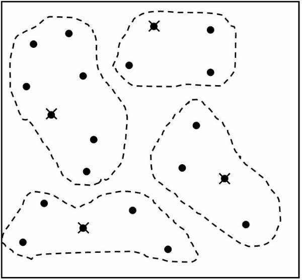
Figure 4.3-1 Randomly Selected Objects
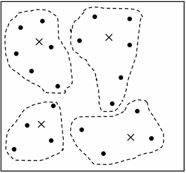
Figure 4.3-2 Redistribution of the Objects
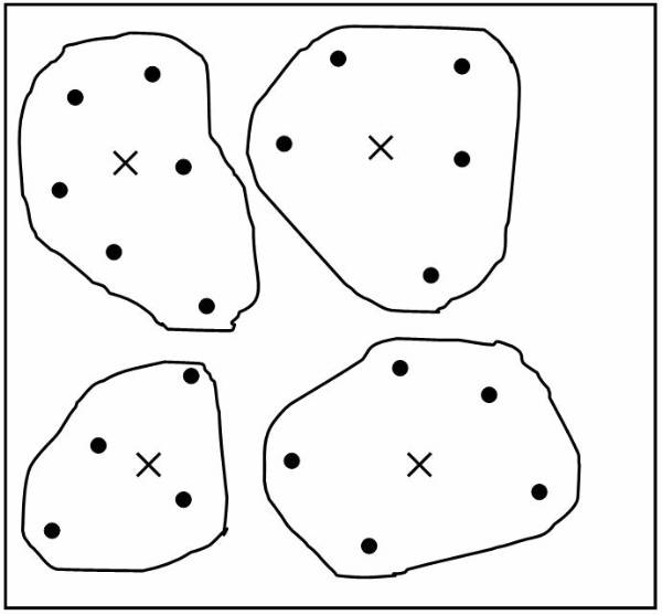
Figure 4.3-3 Final Clusters
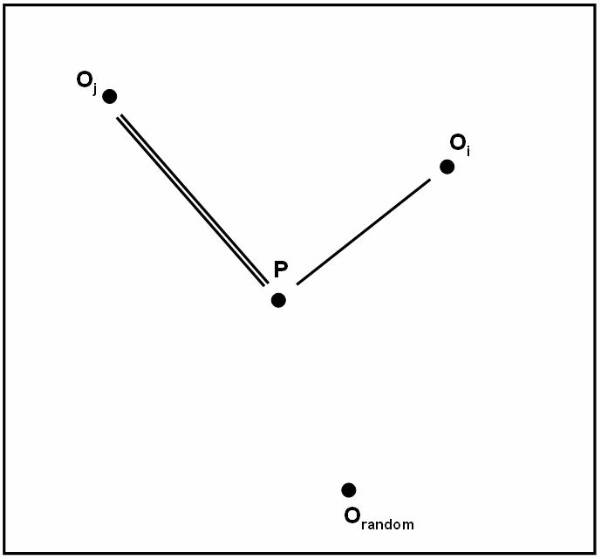
Figure 4.3-4 Reassignment to Oj
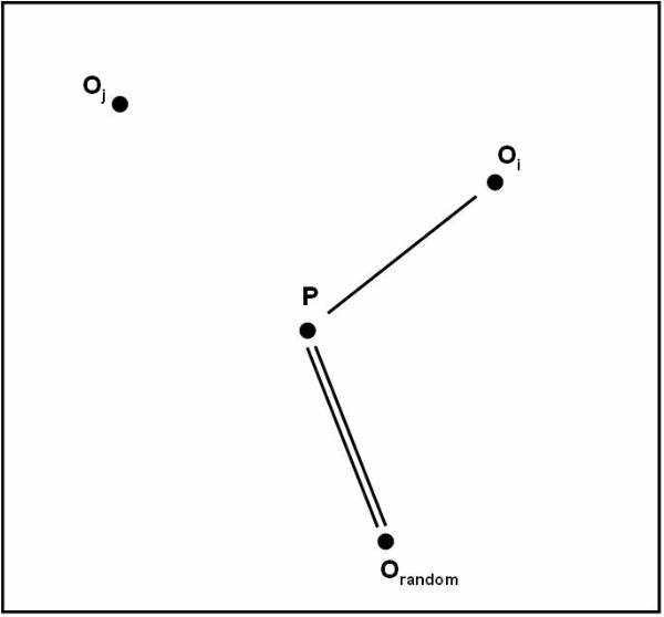
Figure 4.3-5 Reassignment to Orandom
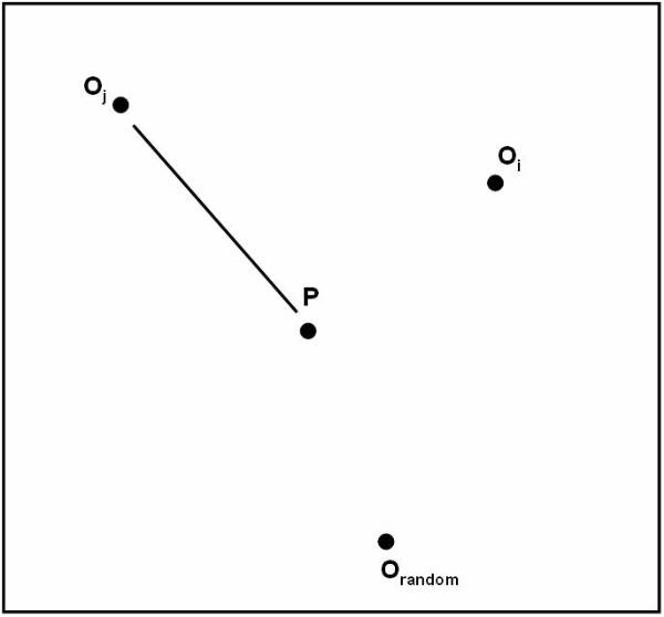
Figure 4.3-6 No Change in Object Positions
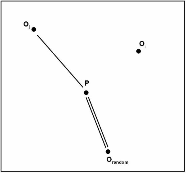
Figure 4.3-7 Reassignment to Orandom
Hierarchical Method
Hierarchical method groups all the objects into a tree of clusters that are arranged in hierarchical manner. It works on bottom-up or top-down approaches.
Agglomerative and Divisive Hierarchical Clustering
Agglomerative hierarchical clustering method works on the bottom-up appoach. In this method each object creates its own clusters. The single clusters are merged to make larger cluster and the process of merging continues until all the singular clusters are merged into one big cluster that consists of all objects.
Divisive hierarchical clustering method works on the top-down approach. In this method all the objects are arranged within a big single cluster and the large cluster is continuously divided into smaller cluster until each cluster has a single object.
Consider a data set, which consists of six data
objects, such as 1, 2, 3, 4, 5 and 6. This figure ![]() shows the agglomerative application AGNES
(AGglomerative NESting) and divisive application DIANA (DIvisive ANAlysis). In
AGNES, each object creates a singular cluster and the clusters are then merged
level-by-level according to minimum Euclidean Distance. This process continues
until all the singular data objects are merged into a big single cluster. In
DIANA, all objects are arranged in a single cluster, and this single cluster is
divided into smaller clusters according to maximum Euclidean distance and this
process continues until each cluster has only one object.
shows the agglomerative application AGNES
(AGglomerative NESting) and divisive application DIANA (DIvisive ANAlysis). In
AGNES, each object creates a singular cluster and the clusters are then merged
level-by-level according to minimum Euclidean Distance. This process continues
until all the singular data objects are merged into a big single cluster. In
DIANA, all objects are arranged in a single cluster, and this single cluster is
divided into smaller clusters according to maximum Euclidean distance and this
process continues until each cluster has only one object.
In both hierarchical clustering methods, user can specify the desired number of cluster as a termination condition. There are four distances used to measure the distance between two clusters. In O and O' represents two objects that are contained by clusters Ci and Cj, Mi is the mean for Ci, and Ni is the number of objects in Ci, then distances are:
Minimum Distance:
![]()
Maximum Distance:
![]()
Mean Distance:
![]()
Average Distance:
![]()
The main drawback of the hierarchical method is regarding the selection of merge or split points. Once the clusters are merged or a cluster is divided into smaller clusters, the generated clusters can not be changed. It can not be undone what was done and also swapping between clusters can not be perform.
Balanced Iteractive Reducing and Clustering Using Hierarchies (BIRCH)
BIRCH is another type of hierarchical clustering method that depends upon two features, clustering feature (CF) and clustering feature tree (CF tree). Both of them represent all objects into clusters as hierarchical representation.
CF is a triplet function that contains the information about sub-clusters of objects. CF of the sub-cluster, which contains a multi-dimensional object Oi, is defined as:
![]()
where N represents the number of objects in a sub-cluster, LS represents the linear summation of N objects,
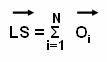
and SS represents the square of summation of N data objects.
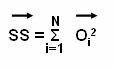
A CF tree is a height-balanced tree, which
consists of clustering feature to represent the clusters in hierarchical
representations. This figure ![]() shows the structure of CF tree, which contains
k clustering features in each sub-cluster and each objects have k children.
Root node has one sub-cluster with k objects and level 1 node consists of k
sub-clusters with k objects. The BIRCH method works as:
shows the structure of CF tree, which contains
k clustering features in each sub-cluster and each objects have k children.
Root node has one sub-cluster with k objects and level 1 node consists of k
sub-clusters with k objects. The BIRCH method works as:
BIRCH examines the data set to build an initial in-memory CF tree that represents the multilevel compression of the data objects in the form of clustering features.
BIRCH selects a clustering algorithm to cluster the leaf-nodes of the CF tree. Leaf node does not have any children node.
BIRCH produces the best clusters with available input data set and algorithms and uses multiple techniques, which means that BIRCH examines the data objects two or three times to improve the quality of the built CF tree. The drawback of BIRCH is its suitability only for spherical clusters.
Clustering Using Representatives (CURE)
The clustering algorithms generally work on spherical and similar size clusters. The clustering algorithms are prone and outliers. CURE overcomes the problem of spherical and similar size of cluster and is more robust with respect to outliers.
In CURE, first randomly select a fixed number of representative points instead of one centroid using all scattered objects for cluster. Now move all the representative points towards the cluster centre by using a fraction, shrinking factor. When CURE is used in large data set for clustering, it works as the combination of random sampling and partitioning algorithms. It means, a random sample of object data set is partitioned and each partition is simultaneously partially clustered. Finally these all partially clusters are merged and produce desired cluster as output. The CURE algorithms work on following steps:
Randomly create a sample of all the objects that are contained in a data set.
Divide the sample into definite set of partitions.
Simultaneously create partial cluster in each partitions.
Apply random sampling to remove outliers. If a cluster grows slowly, then delete this cluster from the partition.
Cluster all the partially created clusters in each partition using shrinking factor. It means all the representative points formed a new cluster by moving towards the cluster centre that is specified by user-defined fraction shrinking factor.
Label the formed cluster.
For example, a data set that
contains n objects and cluster is to be made of all the objects using CURE
clustering method. This figure ![]() shows a data set of objects. This sample data
has to be divided into two partitions. The objects within the each partition
are partially clustered using dissimilarity distance measurements. This figure
shows a data set of objects. This sample data
has to be divided into two partitions. The objects within the each partition
are partially clustered using dissimilarity distance measurements. This figure ![]() shows two partitions of the sample data set
and objects in each partition are partially clustered. The centre of clusters
are shown by X symbol.
shows two partitions of the sample data set
and objects in each partition are partially clustered. The centre of clusters
are shown by X symbol.
In each partition, partial
clusters through its representative points are moved towards the cluster centre
using fraction factor. New cluster is begin to start by capturing the shape of
each partial clusters. This figure ![]() shows the movement of all the partial clusters
towards the centre cluster using shrinking factor and capturing their shapes to
form a new cluster in each partition. This figure
shows the movement of all the partial clusters
towards the centre cluster using shrinking factor and capturing their shapes to
form a new cluster in each partition. This figure ![]() shows two clusters of different shapes and
sizes after merging both the partitions into a data set.
shows two clusters of different shapes and
sizes after merging both the partitions into a data set.
Chameleon Method
Chameleon is another hierarchical clustering method that uses dynamic modeling. chameleon is introduced to recover the drawbacks of CURE method. In chameleon clustering method, tow clusters are merged, if the interconnectivity between two clusters is greater than the interconnectivity between the objects within a cluster. These are the steps how chameleon method works:
Construct
a sparse-graph from the data set that consists of n objects. This figure ![]() shows a graphical representation of all the
objects that are contained in a data set.
shows a graphical representation of all the
objects that are contained in a data set.
Divide
a sparse-graph into large number of small sub-clusters using any partitioning
algorithm. This figure ![]() shows the clusters' small size clusters that
are produced after applying the partitioning algorithms.
shows the clusters' small size clusters that
are produced after applying the partitioning algorithms.
Merge
the small size clusters into a big cluster on the basis of chameleon
interconnectivity concepts. This figure ![]() shows the merging of the small clusters into
big cluster, of the interconnectivity between the clusters is greater than the
interconnectivity between the objects with a cluster.
shows the merging of the small clusters into
big cluster, of the interconnectivity between the clusters is greater than the
interconnectivity between the objects with a cluster.
Chameleon calculates the interconnectivity between two clusters Ci and Cj by relative interconnectivity and relative closeness of clusters.
The Relative Interconnectivity (RI): The RI is the ratio of absolute inteconnectivity between two clusters Ci and Cj and the internal interconnectivity of the each cluster.
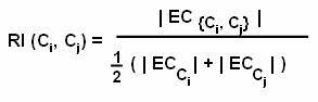
where EC represents the edge-cut of a cluster that containing both clusters. ECCi and ECCj represents the size of min-cut bisector.
The Relative Closeness (RC): The relative closeness is the ratio of absolute closeness between two clusters Ci and Cj and the internal closeness of each cluster.
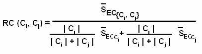
where S'EC is the weight of the edge tha tjoin the vertices if Ci to Cj and S'ECCi or S'ECCj is the weight of the edges that represents the min-cut bisector of each cluster.
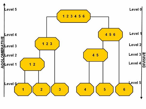
Figure 4.4-1 Agglomerative and Divisive Hierarchical Clustering Methods
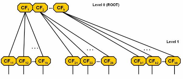
Figure 4.4-2 Tree Structure
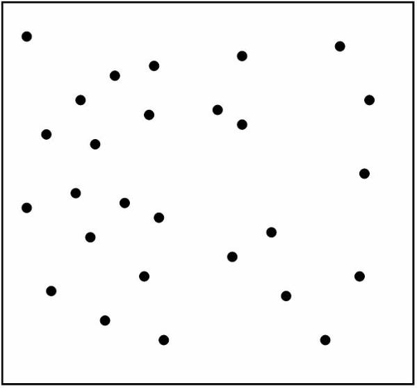
Figure 4.4-3 Sample Data Set with Objects
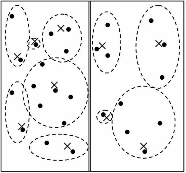
Figure 4.4-4 Partially Clustering in Each Partition
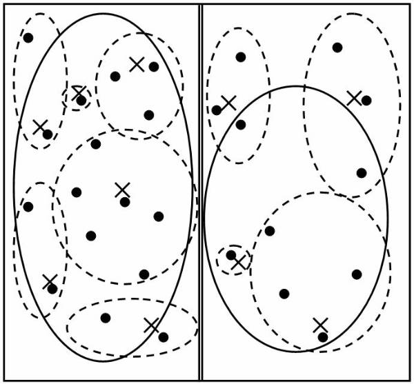
Figure 4.4-5 Shrinking of Partial Clusters towards the Centre Cluster
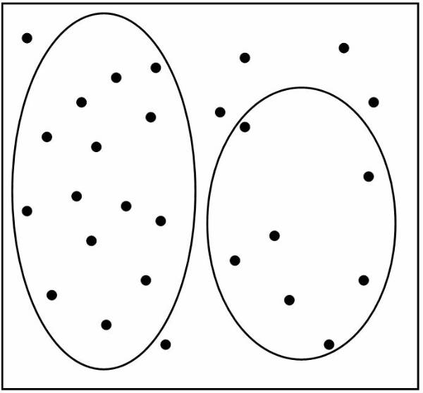
Figure 4.4-6 Output Clusters
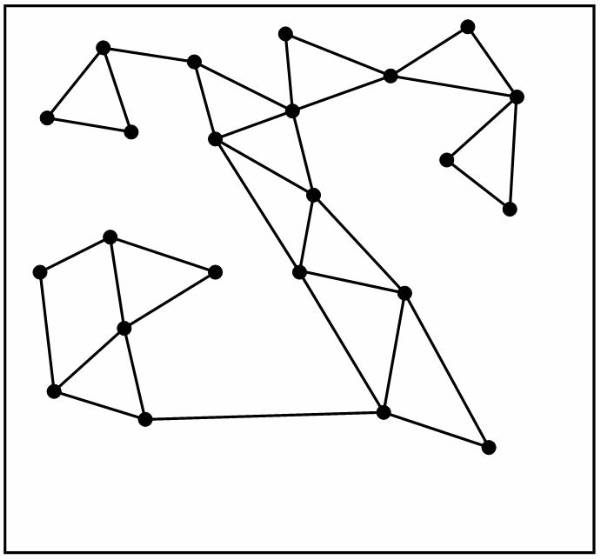
Figure 4.4-7 Construction Sparse-Graph for n Objects
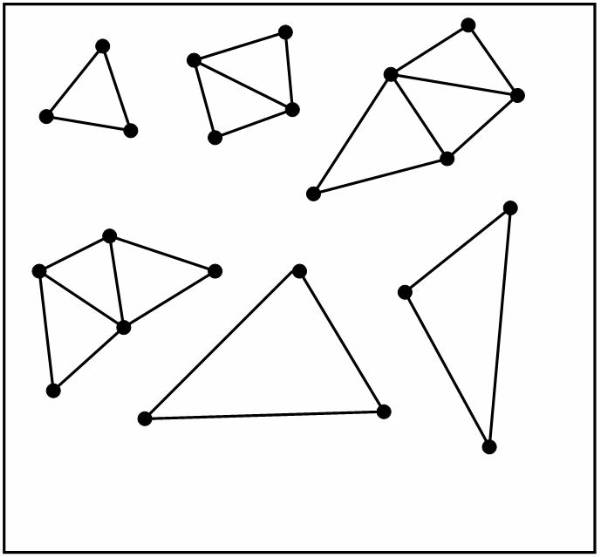
Figure 4.4-8 Partitioning the Sparse-Graph
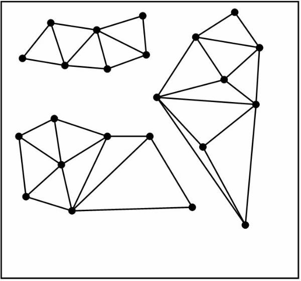
Figure 4.4-9 Margining the Partitions
Density-Based Method
Density-based method deals with arbitrary shaped clusters, in this method, clusters are formed on the basis of the region where density of objects is high.
Density-Based Spatial Clustering of Application Noise (DBSCAN)
DBSCAN is density-based clustering method that converts the high-density objects regions into clusters with arbitrary shapes and sizes. DBSCAN defines the cluster as a maximal set of density-connected points. The basic terms that are used in DBSCAN clustering method are:
The neighbourhood of an object that is enclosed in a circle with radius I is called I-neighbourhood of the object.
I-neighbourhood with minimum object points (MinPts) is called as core object.
An object A, from a data set is directly density-reachable from abject B, where A is the member of I-neighbourhood of B and B is a core object.
DBSCAN works as follows:
Check the I-neighbourhood for each data points in a data set.
Creates core objects, if the I-neighbourhood of this object contains MinPts data points.
Collects all the objects that are directly density-reachable from these core objects.
Merge some of these objects, which are directly density-connected objects, to form new cluster.
Terminate this process, when no other data points can be added to any cluster.
For example, consider a data set that contains
various data points, where value of MinPts = 4 and the specified radius of
circle is I. This figure ![]() shows the density reachability between the
objects. In this figure A, C, D and F are core objects because their I-neighbourhood consists of at
least four data points. B is directly density-reachable from C and C is
directly density-reachable from A. Although B is directly reachable to C and C
is directly reachable to A, but B is indirectly density-reachable from A
because B is not a core object. Here D, E and F all the density-connected
objects. These density-connected objects from a new cluster, called
density-based cluster.
shows the density reachability between the
objects. In this figure A, C, D and F are core objects because their I-neighbourhood consists of at
least four data points. B is directly density-reachable from C and C is
directly density-reachable from A. Although B is directly reachable to C and C
is directly reachable to A, but B is indirectly density-reachable from A
because B is not a core object. Here D, E and F all the density-connected
objects. These density-connected objects from a new cluster, called
density-based cluster.
Ordering Points To Identify the Clustering Structure (OPTICS)
The DBSCAN method of clustering takes as input MinPts and I from the user, and these parameters are sensitive for real life and high-dimensional data. To overcome this problem, OPTICS is introduces. It calculates the clustering order for automatic cluster analysis instead of explicit clustering by user. The cluster ordering represents the density-based clustering structure, which consists of the information that is equivalent to density-based clustering. The basic terms that are used in OPTICS are:
Core Distance: The core distance of and object A is the smallest I' value that makes A core object.
Reachability Distance: The reachability distance of an object A with
respect to object B is the greater value of the core-distance of object B. It
is similar to the Euclidean distance between A and B. For example, consider a
data set that contains various data points. This figure ![]() shows the core and reachability distance
between the objects, where I' is the
core distance of objects A and reachability distance of m with respect to A.
shows the core and reachability distance
between the objects, where I' is the
core distance of objects A and reachability distance of m with respect to A.
The OPTICS method works on the steps:
Creates an order of objects from a data set that stores the core distance and reachability distance of the objects.
Extract clusters on the basis of stored information.
For example, a data set that contains
various clusters and each cluster consists of objects. These clusters are
arranged in a particular order. This figure ![]() shows the reachability plot for a
two-dimensional data set that represents the overview of data structure and
clusters. This method is used to view multi-dimensional clustering structure.
shows the reachability plot for a
two-dimensional data set that represents the overview of data structure and
clusters. This method is used to view multi-dimensional clustering structure.
DENsity-Based CLUstEring (DENCLUE)
DENCLUE is a clustering method based on a set of density distribution functions. The basic terms that are used in this method are:
Each data point from a data set is modelled by using an influence function, which describes the impact of a data point that is enclosed to the neighbourhood.
The overall density of data space is modelled using the sum of the influence functions of all data points.
Clusters are determined mathematically by using density attractors, where density attractors are local maxima of the overall density function.
If x and y are the objects of multi-dimensional feature space, then the influence function of data object y an x is a function
![]()
that is defined as:
![]()
This is the function that is used to measure the distance between two objects. The distance function is similar to Euclidean distance that is used to compute the square wave influence function and Gaussian influence function. The square wave influence functions is defined as:
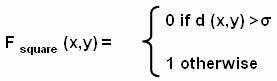
And the Gaussian influence functions is defined as:
![]()
The density function for an object x is the sum of influence functions of all data points. If a data set that consists of n data points such as x1 to xn, then the density function of object x is:
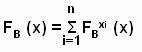
The
density function is used to define the gradient of the function and density
attractor. Figure ![]() shows the two-dimensional data set that contains
various data points. This figure
shows the two-dimensional data set that contains
various data points. This figure ![]() shows a square wave function as the output for
a given two-dimensional data set. This figure
shows a square wave function as the output for
a given two-dimensional data set. This figure ![]() shows a Gaussian wave function as the output
for a give data set.
shows a Gaussian wave function as the output
for a give data set.
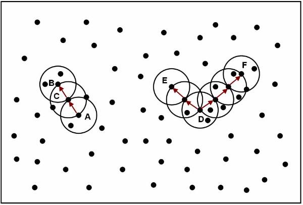
Figure 4.5-1 Density Reachability in Density-Based Clustering
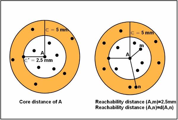
Figure 4.5-2 he Core Distance and Reachability Distance
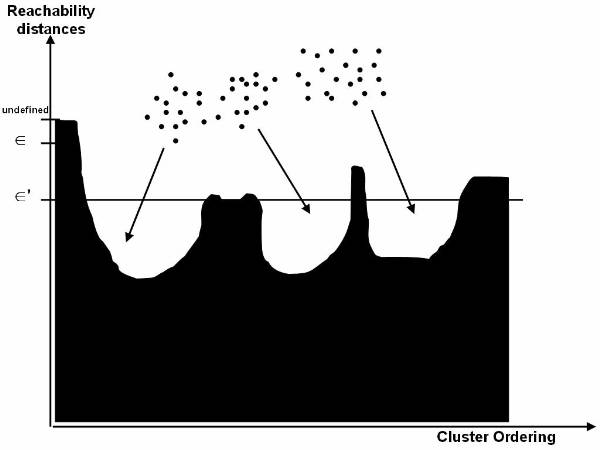
Figure 4.5-3 Graphical Representation of Data Object Ordering
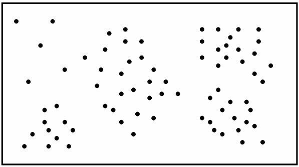
Figure 4.5-4 Two-Dimensional Data Set
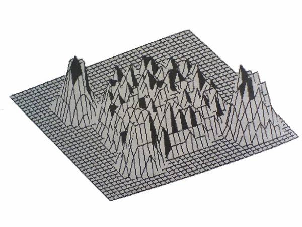
Figure 4.5-5 Square Wave Function
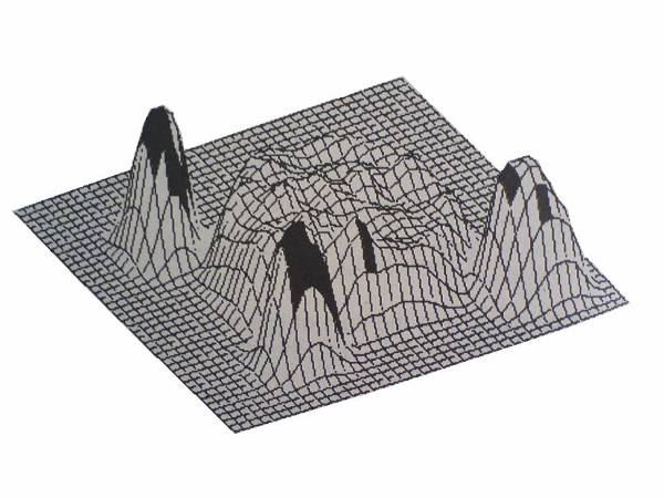
Figure 4.5-6 Gaussian Wave Function
Grid-Based Method
In grid-based method, objects are represented by the multi-resolution grid data structure. All the objects are quantized into a finite number of cells and the collection of cells build the grid structure of objects. The clustering operations are performed on that grid structure. This method is widely used because its processing time is very fast and that is independent of number of objects.
STatistical INformation Grid (STING)
STING is a grid-based multi-resolution
clustering method, in which all the objects are contained into rectangular
cells, these cells are kept into various levels of resolutions and these levels
are arranged in a hierarchical structure. Each cell in a higher level is
divided into a number of cells at the lower level. Each cell stores the
statistical information of each objects and this statistical information is
used in query processing. This figure ![]() shows the hierarchical representation, the n
levels, cells in each higher level divides into number cells at next lower
level. A statistical parameter of higher level is calculated with the help of
lower level statistical parameters. Each cells contains the attribute
independent parameter such as count, attribute dependent parameters such as
mean (M), standard deviation (s), minimum (MIN), maximum (MAX) and types of
data distribution such as normal, uniform, exponential, or none. Distribution
of data is specified by user or hypothesis tests such as X2 and it is measured by the majority of
the lower level cells.
shows the hierarchical representation, the n
levels, cells in each higher level divides into number cells at next lower
level. A statistical parameter of higher level is calculated with the help of
lower level statistical parameters. Each cells contains the attribute
independent parameter such as count, attribute dependent parameters such as
mean (M), standard deviation (s), minimum (MIN), maximum (MAX) and types of
data distribution such as normal, uniform, exponential, or none. Distribution
of data is specified by user or hypothesis tests such as X2 and it is measured by the majority of
the lower level cells.
Wave Cluster
The wave cluster is a type of grid-based multi-resolution method, in which all the objects are represented by a multidimensional grid structure and a wavelet transformation is applied for finding the dense region. Each grid cell contains the information of a group of objects that map into a cell. A wavelet transform is a process of signalling that produces the signal of various frequency sub-bands.
This figure ![]() shows a two-dimensional sample feature space.
In this figure each pixel of the image represents the value of the one data
object. When wavelet transformation is applied at different resolution from
high to low level resolution, the two-dimensional feature space is changed.
Figure
shows a two-dimensional sample feature space.
In this figure each pixel of the image represents the value of the one data
object. When wavelet transformation is applied at different resolution from
high to low level resolution, the two-dimensional feature space is changed.
Figure ![]() shows the sample of two-dimensional feature
space at different resolution levels, the three scales from 1 to 3, scale 1
shows the feature space in high resolution, scale 2 shows the space feature in
medium resolution and scale 3 shows the space feature in low resolution.
shows the sample of two-dimensional feature
space at different resolution levels, the three scales from 1 to 3, scale 1
shows the feature space in high resolution, scale 2 shows the space feature in
medium resolution and scale 3 shows the space feature in low resolution.
Wavelet-based clustering technique is used because it supports unsupervised clustering and supports the multi-resolution property of wavelet transformation. As a result, clusters are detected from different level of accuracy and it is the fastest algorithm.
Clustering in QUEst (CLIQUE)
The Clique is an integrated version of density-based and grid-based clustering methods and it is generally used in large data set. All the object points of a large data set are uniformly distributed in data space and CLIQUE represents the crowded area of object points as unit. A unit is dense, if the fraction of data points is exceeds an input model parameter. The CLIQUE method works as follows:
Partitions the multi-dimensional data space into non-overlapping rectangular units representing the dense unit.
Generates a minimal description for each cluster.
For example, a data set consists
of employee's information such as age, experience and salary. This figure ![]() shows the dense rectangular units,
where X-axis represents the age of the employee and Y-axis represents the
salary of the employee. Figure
shows the dense rectangular units,
where X-axis represents the age of the employee and Y-axis represents the
salary of the employee. Figure ![]() shows the rectangular units, where X-axis
represents the age of the employee and Y-axis represents the working experience
of the employee.
shows the rectangular units, where X-axis
represents the age of the employee and Y-axis represents the working experience
of the employee.
Now CLIQUE form a candidate search space by intersecting these two dense units representing sub-spaces . A candidate search space represents the dense units with higher dimensionalities.
This figure ![]() shows a three-dimensional rectangular, in
which X-axis represents the age, Y-axis represents the experiences and Z-axis
represents the salary.
shows a three-dimensional rectangular, in
which X-axis represents the age, Y-axis represents the experiences and Z-axis
represents the salary.
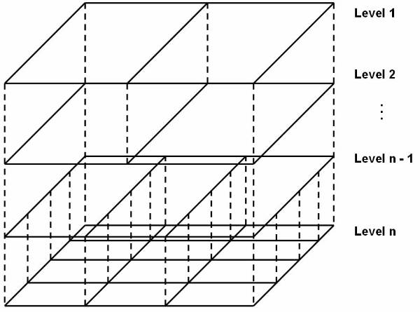
Figure 4.6-1 A Hierarchical Structure Using STING

Figure 4.6-2 A Sample of Two-Dimensional Feature Space
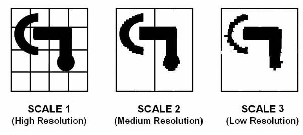
Figure 4.6-3 Multi-resolution of the Two-dimensional Feature Space
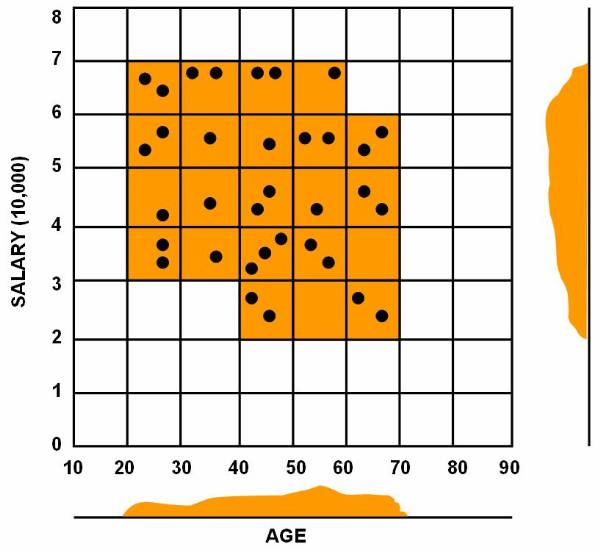
Figure 4.6-4 Rectangular Units with respect to Age and Salaries
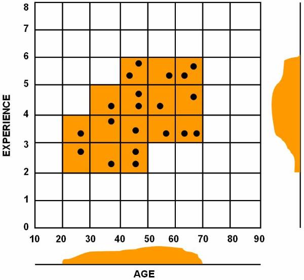
Figure 4.6-5 Rectangular Units with respect to Age and Experience
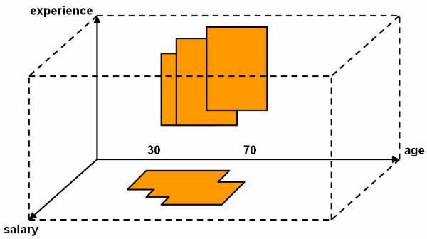
Figure 4.6-6 A Candidate Space Representation
Model-Based Method
The model-based clustering method is used for optimising the fit between a given data set and a mathematical model. The model-based method uses an assumption that the data are distributed by probability distributions. There are two basic approaches of model-based method, statistical method and neural network method.
Statistical Approach
Statistical clustering method is used for conceptual clustering that is also type of clustering. In this conceptual clustering, a set of unlabeled objects is presented in by classification tree. Conceptual clustering groups the objects into concept or class and that class also contains the characteristics descriptions of the group.
Statistical approach uses probability
measurements to determine the concepts of cluster. COBWEB is a clustering
method that uses the concept of statistical approach. COBWEB constructs a
hierarchical classification tree of clusters. For example, a data set of
automobile that contains the information about two-wheeler, three-wheeler and
four-wheeler. This figure ![]() shows a classification tree, in which data
automobile is represented as its root node and each node represents the
concepts or class that contains the probabilistic description of the class
objects. The probabilistic description includes probability of the concept and
conditional probability, which is:
shows a classification tree, in which data
automobile is represented as its root node and each node represents the
concepts or class that contains the probabilistic description of the class
objects. The probabilistic description includes probability of the concept and
conditional probability, which is:
![]()
Where, Ai = Vij represents the attribute value pair and Ck represents the concept or class. COBWEB method uses a category utility to construct the classification tree. Category utility is a heuristic evaluation measure that is defined as
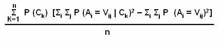
Where n is the number of nodes that forms the partitions from C1 to Cn at a particular level. The classification tree is constructed on the basis of interclass dissimilarity and intra-class similarity.
Neural Network Approach
In neural network approach for clustering, clusters are represented as exemplar. An exemplar is a prototype of a cluster. New objects are distributed to a cluster on the basis of some distance measure. There are two clustering methods that follows the neural approach, competitive learning and self-organizing feature maps.
A competitive learning method represents a
hierarchical architecture of various units or neurons. In this method all the
neurons compete in a winner-takes-all manner. This figure ![]() shows the competitive learning model, in which
each layer consists of several units that are shown by circle and each unit
consists of active and inactive winning points. Active winning points are
represented by filled circle and inactive winning points are represented by
symbol X. The interconnection between layers is called excitatory. A unit
receives input from the lower level. The active winning points in a layer
represent the input pattern for higher layer.
shows the competitive learning model, in which
each layer consists of several units that are shown by circle and each unit
consists of active and inactive winning points. Active winning points are
represented by filled circle and inactive winning points are represented by
symbol X. The interconnection between layers is called excitatory. A unit
receives input from the lower level. The active winning points in a layer
represent the input pattern for higher layer.
Self-organizing feature maps (SOM) is also represented by competition of various units for the current object. The units whose weight vector is similar to the current objects becomes the winning or active unit.
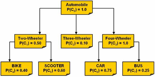
Figure 4.7-1 A Classification Tree of Automobile Data Set
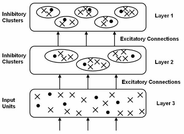
Figure 4.7-2 A Competitive Learning Model
Introduction to Association Rules
Association rules is a process to search relationships among data items in a given data set, which helps in managing all the data items. Association rules are used when a data set has large data items. For example, a departmental store keeps a record of daily transactions where each transaction represents the items bought during one cash register transaction by a person. The manager of the departmental store generate the summarized report of the daily transactions that includes the information about what types of item have sold at what quantity. This report also includes the information about those products, which are generally purchased together. Suppose the manager made a rule, if a person purchases the bread then he also purchase the butter. As a result, when availability of bread declines, probably the stock of butter also declines. The manager can make these types of checks using association rules.
Basic Terminology
Before studying the basic algorithms, it is necessary to know the basic terminologies that are used to search the association rules among a given data set. When association rules are searched, various types of notations an terms are used. The important notations and their meanings are:
D: Database of transactions
ti: Transaction in D
s: Support
a: Confidence
X, Y: Itemsets
X Þ Y: Association Rules
L: Set of large itemsets
I: Large itemset in L
C: Set of candidate itemsets
p: Number of partitions
The basic terms of association rules are:
Association Rules: Let a data set I = and a database of transaction D = where ti = and Iij I I. Association rule is an implication of the form X Þ Y where X, Y Ì I are items of data set called as itemsets, and X Y = F
Support: The support for an association rule X Þ Y is the percentage of transaction in the database that consists of X È Y.
Confidence: the confidence for an association rule X Þ Y is the ratio of the number of transactions that contains X È Y to the number of transaction that contains X.
Large Item Set: A large item set is an item set whose number of occurrences is above a threshold or support. L represents the complete set of large itemsets and I represents an individual item set. Those large itemsets that are counted from data set are called as candidates and the collection of all these counted large itemsets are known as candidate item set.
Association rule are searched from the large data set by using the two steps:
Find the large item set from the given data set.
Generate the association rules from the large itemsets.
Various types of algorithms can be used to find the large item set from the data set. Once the large itemsets are found, the association rules can be generated. This pseudo code shows how to generate the association rule from the large itemsets:
Input:
D // Database of transaction
I // Items
L // Large item set
s // Support
a // Confidence
Output:
R // Association rules
Association_Rule_Generate_Procedure:
R
for each 1 I L do
for each X Ì 1 such that X ¹ do
if support (1) / support (X) >= a then
R= R È
end if;
end for;
end for;
Apriori Algorithm
The Apriori algorithm is an association rule algorithm that finds the large itemsets from a given data set. This algorithm is based on the large item-set property, a sub-set of any large item-set must be large. It is used to generate the candidate itemsets of a definite size and then scan the data set for investigating if itemsets are large item set. For example, during ith scan of a data set, candidates of size i, Ci are counted. Only those candidates are passed to next scan of the database that are large, it means Li is used to generate the Ci+1. To generate a candidates of size i+k, the kth size item set is joined to the previous item set. Apriori algorithm generates the candidate itemsets for each scan except first scan because in the first scan all the itemsets are considered as candidates.
For example, a departmental store consists of various types of articles. This table shows 5 cash register transactions of one day:
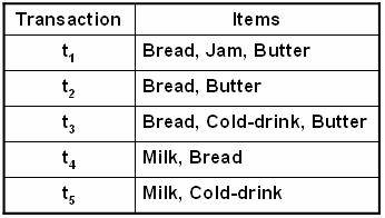
This table shows the candidates and large itemsets after each scan of data set using Apriori algorithm:
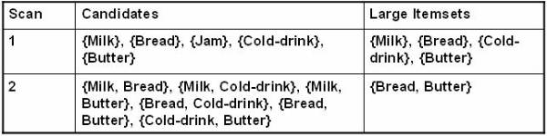
When Apriori algorithms were applied on daily transaction of departmental store, in first scan we get five candidates and only four of them are large. Large candidates are combined with all the other large candidates to form the candidates for the next scan. As a result, the candidates for next scan is (L-1) + (L-2) + 1 = 3 + 2 + 1 = 6 and only 1 candidate out of the lot is large.
This is the pseudo code for generating the candidates of user given size:
Input:
Li-1 // Large itemset if size i - 1
Output:
Ci // Candidates of size i
Apriori_candidate_generation_procedure:
Ci =
for each I I Li-1 do
for each J ¹ I I Li-1 do
if i-2 of the elements in I and J are equal then
Ck = Ck È
end if;
end for;
end for;
The above listing generates the candidates for each scan of database. This is pseudo code for generating the large itemset that are further used to find the association rules:
Input:
I // Itemsets
D // Database of transactions
s // Support
Output:
L // Large itemsets
Apriori_procedure:
k = 0; // Counts the scan number
L =
Ci = I // Initialise the candidate
repeat
k = k + 1;
Lk =
for each Ii I Ck do
Ci =0; // Initiate the counters
for each tj I D do
if Ii I tj then
Ci = Ci+1;
end if;
end for;
end for;
for each Ii I Ck do
if Ci >= ( s* |D|) do
Lk = Lk È Ii;
end if;
L = L È Lk;
Ck+1 = Apriori_candidate_generation_procedure (Lk)end for;
end for;
until Ck+1 =
The Apriori algorithm assumes that the transaction database is memory-resident. The number of database scan is large for Apriori algorithm, which is the main drawback of the Apriori algorithm.
Sampling Algorithm
To overcome the counting of itemset with large data set in each scan, sampling algorithm has to be used. The sampling algorithm reduces the number of data set scan to 1 or 2 where 1 is for the best case and 2 is for the worst case. Sampling algorithm is also used to find the large itemset for the sample from data set like the Apriori algorithm. These samples are considered as Potentially Large (PL) itemset that are used as candidates for counting the entire database. Additional candidates are considered by applying the negative border function (BD_). The entire set of candidates C = PL È BD_(PL). The negative border function is the generalization from the Apriori algorithm. Sampling algorithm uses the Apriori algorithm to find the large itemsets in the sample. The set of large itemsets is used as a set of candidates, when the entire database is scanned. If and itemset, which is present in a sample, is large, then these itemsets are considered as Potentially Large. All the large itemsets are obtained in the first scan of the database using negative border function, if PL is expanded by this negative border function.
In the first scan of the database, all the candidates C are counted. If all the candidates that are only present in PL are large, then all the large items are found in first scan. If some of the large intems are present in negative border function, then the entire database has to be scanned twice. In second scan, some additional candidates are generated and then counted. These additional candidates are added to find the missing large itemsets that are absent in the first scan PL but present in the L. To find all the remaining large itemsets in the second scan, sampling algorithm continuously apply on negative border function until the user gets all missing large itemsets. This pseudo code generates the large itemset from the data set:
Input:
I // Itemsets
D // Database of transactions
s // Support
Output:
L // Large Itemsets
Sampling_procedure:
Ds = Sample drawn from D;
PL = Apriori_procedure (i, Ds, smalls);
L =
for each Ii I C do
Ci = 0; // Initialise the counter
for each tj I D do // First scan
if Ii I tj then
Ci = Ci + 1;
end if;
end for;
for each Ii I C do
if Ci >= (s* |D|) do
L = L È Ii;
end if;
ML = ; // Missing large itemsets
if ML ¹ then
C = L; // Set candidates to be large sets
end if;
end for;
end for;
repeat
C = C È BD_(C); // Expand candidates sets
until no row itemsets are added to C;
for each Ii I C do
Ci = 0;
for each Ii I C do
if Ii I C then
Ci = Ci + 1;
end if;
if Ci >= ( s * |D| ) do
L = L È Ii;
end if;
end for;
end for;
The Apriori algirithm is applied to the sample to find the large itemset using a support called smalls. The smalls can be any support value less then s. For example, departmental stores have various articles in stores and use sampling algorithm to find all large itemsts in the grocery data, where s = 20%. Let the sample database consists of two transactions,
Ds =
If s is reduced to 10%, then an itemset is large in the sample when this itemset occurs in at least 0.1 x 2 transaction. It means that itemset should occur in one of the two transactions. The value of PL when apriori is applied on the Ds is,
PL =
After applying the negative border fiunction on the PL, we get,
BD_(PL) =
The set of candidates for first scan of the database,
PL=
For an itemset to be large it is compulsory that an itemset in 0.2 x 5 or at least one transaction. Milk and Cold drink are both large. Then,
ML=
When the negative border is applied if C is equal to PL, then we get,
C = BE_(C) =
This also has some uncovered item sets, so this algorithm is again applied until all the itemsets are of the size three.
Partitioning Algorithm
In partitioning algorithm, the database of transaction D is divided into k partitions, such as D1, D2, , Dk. The partition algorithm divides the database of transaction in such way that the scan of database is reduced to two scan and each partition can be placed into main memory. When the database is scanned, partition algorithm places the appropriate partition into the main memory and counts the item in that particular partition. The Apriori algorithm can be used for finding the large itemset from each partition. In partitioning algorithm, Li represents the large itemsets that are taken from the Di partition.
In the first scan of the database, the partitioning algorithm finds all large items set in each partition. In the second scan of the database, only those itemsets, which are large and present in at least one partition, are used as candidates. The candidates are counted to determine if they are large across the entire database. This is the pseudo code for generating the large itemsets using partitioning algorithm:
Input:
I // Itemsets
D = // Divides into k partitions
s // Support
Output:
L // Large itemsets
Partition_procedure:
C =
for i=1 to k do // Find the large itemset in each partition
Li = Apriori_procedure (I, Di, s);
C = C È Li;
L =
for each Ii I C do
Ci = 0; // Initialise counts for each itemsets are 0
end for;
for each tj I D do // Count candidates during second scan
for each Ii I C do
if Ii I tj then
Ci = Ci + 1;
end if;
end for;
for each Ii I C do
if Ci >= (s * |D|) do
L = L È Ii;
end if;
end for;
end for;
end for;
The above pseudo code for partitioning algorithm that is using market basket data. For example, a daily transaction report of a departmental store consists of five transactions,
t1 =
t2 =
t3 =
t4 =
t5 =
When the partition algorithm is applied on the above transaction report, database of the transaction is divided into two partitions, D1 and D2,
D1
t2 =
D2
t4 =
t5 =
Let the value of support s = 10%, then the resulting itemsets L1 and L2 are:
L1 =
L2 =
If the items are uniformly distributed into the partitions, then a large fraction of the itemsets will be large. And if the items are not uniformly distributed into the partitions, then there are many false candidates.
Parallel and Distributed Algorithms
The parallel algorithm can be made either attempting the parallelism over the data or candidates. When the user attempt the parallelism over the data, it is called as data parallelism, and when you attempt the parallelism over candidates, it is called task parallelism. In data parallelism, only initial candidates and the local counts at each iterations must be distributed, while in the task parallelism, not only the candidate but also set of transactions must be broadcast to all other partitions.
Count Distribution Algorithm
The Count Distribution Algorithm (CDA) is data parallelism algorithm. CDA divides the database of transaction into k partition, and allocate one processor for each partition. Now, each processor counts the candidates and then delivers these counts to all other processor. This pseudo code generates the large itemset using data parallelism:
Input:
I // Itemsets
P1, P2, , Pk // Processors
D = D1, D2, , Dk //Divided into k partitions
s //Support
Output:
L // Large Itemsets
Count_distrubution_procedure:
Perform in parallel at each processor P1, // Count in parallel
k = 0;
L =
C1 = I;
repeat
k = k + 1;
Lk =
for each Ii I Ck do
Ci1 = 0;
for each tj I D1 do
for each Ii I Ck do
if Ii I tj then
Ci1 = Ci1 + 1;
broadcast Ci1 to all other processors;
end if;
if Ci > ( s * |D1 È D2 È È Dk |) do
Lk = Lk È Ii;
Ck+1 = Apriori_procedure (Lk)
end if;
end for;
end for;
end for;
until Ck+1 =
For example, a departmental store keeps various
things. Figure ![]() shows the CDA algorithm approach in the
departmental stores, there are three processors in this figure. The first processor
P1 counts the first tow transactions, the next processor P2 counts the next two
transactions, and last third processor P3 counts the last transaction. When the
CDA obtains the local counts of any partition, they are broadcast to the other
partitions so global counts may be generated.
shows the CDA algorithm approach in the
departmental stores, there are three processors in this figure. The first processor
P1 counts the first tow transactions, the next processor P2 counts the next two
transactions, and last third processor P3 counts the last transaction. When the
CDA obtains the local counts of any partition, they are broadcast to the other
partitions so global counts may be generated.
Data Distribution Algorithm
The Data Distribution Algorithm (DDA) is a task parallelism algorithm. In the task parallelism algorithm, all the candidates are partitioned among the processors. Each processor in parallel counts the candidates given to it using its local database partition. Task parallelism algorithm use Ck1 to indicate the candidates of size k examined at processor P1. Then each processor broadcasts its database partition to all other database partitions. Each processor then determines large itemsets and generates the next candidates. These candidates divides among the processors for the next scan of the database. This pseudo code is generating the large itemsets using task parallelism:
Input:
I // Itemsets
P1, P2, , Pk // Processors
D = D1, D2, , Dk // Divided into k partitions
s // Support
Output:
L // Large itemsets
Data_distrubution_procedure:
C1 =I;
for each 1 < k do // Distribute size 1 candidates to each processor
determine Ci1 and distribute to P1;
k=0;
L =
repeat
k = k + 1;
Lk =
for each Ii I Ck1 do
Ci1 = 0;
end for;
for each tj I D1 do
for each Ii I Ck1 do
if Ii I tj then
Ci1 = Ci1 + 1;
broadcast Ci1 to all other processors;
end if;
end for;
end for;
for every other processor m ¹ 1 do
for each Tj I Dm do
for each Ii I Ck1 do
if Ii I tj then
Ci1 = Ci1 + 1;
end if;
if Ci > ( s * |D1 È D2 È È Dk|) do
Lk = Lk È Ii;
broadcast Lk1 to all other processors;
Lk = Lk1 È Lk2 È È Lkp
Ck+1 = Apriori_procedure (Lk)
Ck+11 Ì Ck+1;
end if;
end for;
end for;
end for;
until Ck+11 =
The above pseudo code generates the large items
set using task parallelism. For example, a departmental store keeps the various
things. Figure ![]() shows the DDA algorithm approach in the
departmental stores, where are there processors. The first processor P1 counts
Milk and Bread, the next processor P2 counts the Jam and Cold-drink, and the
last processor P3 counts the Butter. When DDA obtains the local counts of any
partition, they are broadcasted to the other partitions so each partition may
obtain the global counts.
shows the DDA algorithm approach in the
departmental stores, where are there processors. The first processor P1 counts
Milk and Bread, the next processor P2 counts the Jam and Cold-drink, and the
last processor P3 counts the Butter. When DDA obtains the local counts of any
partition, they are broadcasted to the other partitions so each partition may
obtain the global counts.
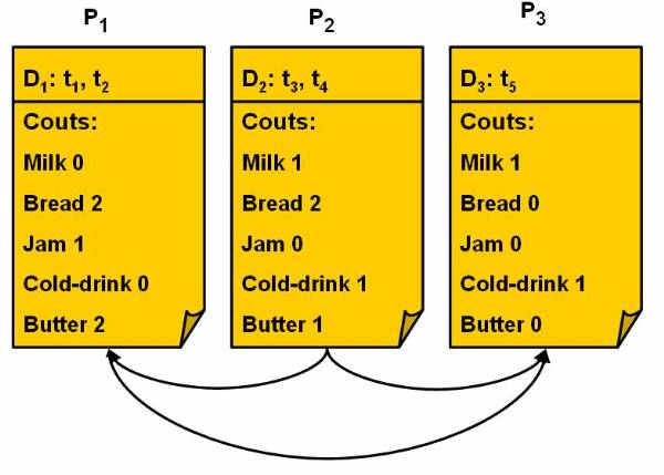
Figure 5.2-1 Data Parallelism Using CDA
Data Parallelism Using CDA (Count Distribution Algorithm)
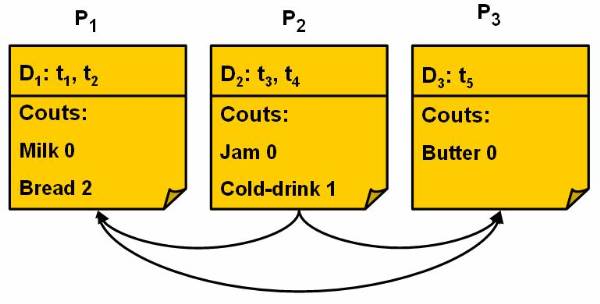
Figure 5.2-2 Data Parallelism Using DDA
Data Parallelism Using DDA (Data Distribution Algorithm)
Comparing the Algorithms
This chapter explained many association rule algorithms. The user needs to know the various factors to decide which algorithm is most suitable for his data set. These are the various factors:
Target: Algorithms should generate all association rules and these rules should satisfy the support and confidence level of the data set.
Type: Algorithms may generate the regular or advanced association rules such as the multiple-level association rules, the quantitative association rules, generalization association rules or constrained based association rules.
Data Type: Algorithms generate the association rules for the various types of data such as plain text and categorical data.
Technique: Using the common techniques such as, Apriori, sampling or partitioning for generating the association rules.
Itemset Techniques: Itemsets can be counted in various ways. The user choose such technique so that all itemsets are generated collectively and then counted.
Transaction Techniques: For counting the itemsets, database of the transaction is scanned. Algorithms count all the transactions that are present in entire data set, a particular sample, or a particular partition.
Itemset Data Structure: Generally all the algorithms use hash tree data structure to store the candidate item sets and their counts. A hash tree is a search tree where each branch that is taken from a level is determined by applying a has function. A leaf node in the hash tree consists of all the candidates that are hashed to it. All the candidates that are present in a leaf are stored in sorted order.
Transaction Data Structure: All the transactions are represented in a flat file or a TID list that is viewed as an inverted file. Gerenaly, all the transactions are encoded by the numbers, letters or symbols.
Architecture: Algorithms are proposed by sequential, parallel and distributed architecture.
Parallelism Techniques: Algorithms use parallelism by two way either data parallelism, or task parallelism. This table shows the comparison of association rule algorithms:
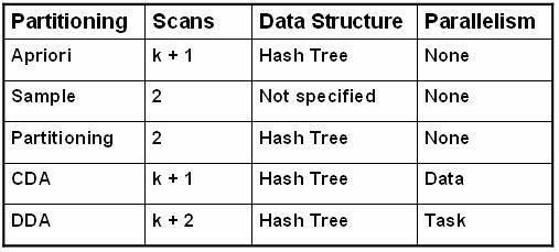
Where k is the number of items, k+1 is the maximum number of scans for the level-wise algorithms.
Association Rules
Association analysis is the discovery of the association rules, which are used for displaying attribute values and conditions that occur frequently in the set of data. In this section the various association rules will be discussed.
Generalized Association Rules
Concept hierarchy is a technique showing the relationship between the various items in the database. Using a concept hierarch in depicting data in the database allows formulation of general rules at each step of the structure. Consider the example of environment around, it is classified as living and non-living; living is further classified into animals, plants and insects; and these are further classified. This classification helps formulation of rules at various levels of the tree structure.
Figure ![]() shows the concept hierarchy in environment.
The generalized association rule is defined as:
shows the concept hierarchy in environment.
The generalized association rule is defined as:
![]()
X Þ Y means that no item Y is above in the hierarchy than X. When The generalized association rule is generated, the user generates all possible rules for that set of node.
Multiple-Level Association Rules
Altering the generalized rules makes the multiple level association rules. With multiple level association rules item sets are picked up from anywhere in the hierarchy. In concept hierarchy, it is based on the top-down approach and large item sets are generated.
Figure ![]() shows the levels in the tree structure for the
environment example. Large itemsets are found at a certain level I and then
there are large itemsets formed at level I+1. This suggests that the size of
itemsets at level zero will be greater than that at level one and so on. As a
result, the minimum support required for the association rules vary based on
the hierarchy level. Now the reduced minimum support concept is based on two
rules:
shows the levels in the tree structure for the
environment example. Large itemsets are found at a certain level I and then
there are large itemsets formed at level I+1. This suggests that the size of
itemsets at level zero will be greater than that at level one and so on. As a
result, the minimum support required for the association rules vary based on
the hierarchy level. Now the reduced minimum support concept is based on two
rules:
Minimum support for all nodes at the same level in the concept hierarchy should be equal.
If Aj, the minimum support for a node at the level i and the minimum support for a node at level i-1 is Ai-1, then Ai-1 > Ai.
Quantitative Association Rules
The generalized and multiple-level association approaches were based on the assumption that the data to be classified is in a categorical form. The quantitative association rules is formed for classifying data, which involves categorical and quantitative data. This pseudo code the items are divided into the several itemsets:
Input:
Items // Input itemsets
p1, p2, p3, , pn // Processors available
d1, d2, d3, , dn // Database divisions
Output:
Large // Larger itemsets
Steps_for_classification:
for each Kj I Items // Partitioning items
if Kj is to be partitioned then
determine the number of partitions that can be made
map the attribute values into new partitions
end if;
replace Kj in Items;
end for;
Using Multiple Minimum Supports
If a database consists of large amount of data items of different types, then there is a problem in defining one minimum support value. Different data items behave differently such as the data arrival trends may be different. Consider a case of data arrival where three different types of data items are being updated to the database. The trends may differ as one entity may increase, one may decrease and the third may fluctuate between two extremes.
As it is emphasized in the example that if there are only two values for an attribute then it is easier to obtain a threshold as compared to a situation, where there is an infinite range of data values. For example, if the rule is formulated as
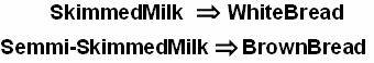
it is easier to find a rule of the above type as compared to the rule
![]()
This suggests that having one general rule is not helpful always. This is a case considering a relatively smaller database but the association rule generation becomes complex in the case of larger databases. This problem with large database is known as rare item problem.
If the minimum support is high then there is a problem that the rules involving items that occur rarely in the database are rarely generated. If the minimum support is low then there is a problem that too many rules are generated. To remove this problem there are different approaches, such as partitioning the database into segments and then generate association rules for each segment separately. The user can also group the rarely occurring items together, separately from rest of the database and then generate rules for the rarely occurring data and the rest data separately and then club then together.
The Correlation Rules
The correlation rule is defined as a set of itemsets, which are connected or correlated. The correlation rules can be developed, because the negative correlation is required in some cases.
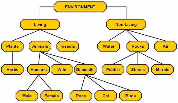
Figure 5.4-1 Concept Hierarchy
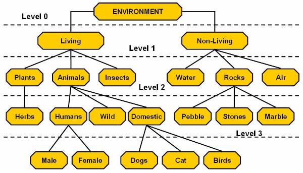
Figure 5.4-2 Levels in Concept Hierarchy
|
Politica de confidentialitate | Termeni si conditii de utilizare |

Vizualizari: 4527
Importanta: ![]()
Termeni si conditii de utilizare | Contact
© SCRIGROUP 2025 . All rights reserved