| CATEGORII DOCUMENTE |
| Bulgara | Ceha slovaca | Croata | Engleza | Estona | Finlandeza | Franceza |
| Germana | Italiana | Letona | Lituaniana | Maghiara | Olandeza | Poloneza |
| Sarba | Slovena | Spaniola | Suedeza | Turca | Ucraineana |
Technical University of ClujNapoca
Faculty of Electronics, Telecommunications and Information
Technology
Semester Project: Antennas & Propagation
Propagation Models in Wireless Systems
Land-mobile communication is burdened with particular propagation complications compared to the channel characteristics in radio systems with fixed and carefully positioned antennas. The antenna height at a mobile terminal is usually very small, typically less than a few meters. Hence, the antenna is expected to have very little clearance, so obstacles and reflecting surfaces in the vicinity of the antenna have a substantial influence on the characteristics of the propagation path. Moreover, the propagation characteristics change from place to place and, if the mobile unit moves, from time to time. Thus, the transmission path between the transmitter and the receiver can vary from simple direct line of sight to one that is severly obstructed by buildings, foliage and the terrain. [1]
Propagation models are fundamental tools for designing any fixed broadband wireless communication system. A propagation model basically predicts what will happen to the transmitted signal while in transit to the receiver. In general, the signal is weakened and distorted in particular ways and the receiver must be able to accommodate the changes, if the transmitted information is to be successfully delivered to the recipient. The design of the transmitting and receiving equipment and the type of communication service that is being provided will be affected by these signal impairments and distortions. The role of propagation modeling is to predict the system performance with these distortions and to determine whether it will successfully meet its performance goals and service objectives. If the performance is inadequate, the system design can be modified accordingly before the system is built.
Traditionally, propagation models is the term applied to those algorithms and methods used lo predict the median signal level at the receiver. Early communication systems were narrowband systems in which median signal level prediction along with some description of signal level variability (fading) statistics were the only models needed to adequately predict system performance. Modern communication systems achieve higher capacity (higher data rates) by using a wider band of frequencies. For such systems, narrowband prediction of signal levels and fading alone does not provide enough information to predict system performance. As a consequence, the concept of a propagation model has been broadened to include models of the entire transfer function of the channel. These models are intended to represent all the modifications the transmitted signal undergoes in traveling from the transmitter to the receiver. Such models include signal level information, signal time dispersion information and in the case of mobile systems, models of Doppler shift distortions arising from the motion of the mobile. Appropriately, such models that provide this additional information are called channel models. [4]
A large number of propagation prediction models have been developed for various terrain irregularities, tunnels, urban streets and buildings, earth curvature, etc. For propagation models addressing satellite communications systems, on the other hand, different types of issues including rain attenuation and atmospheric effects are routinely considered. The level of sophistication in the development of these models also depends on the longevity of the related technology. For example, the importance of developing propagation models suitable for satellite communications, and in particular the development of reliable models for rain attenuation and other atmospheric impairments along earth-satellite paths, has long been recognized; and extensive research activities have been focused on addressing these effects. [2]
1. Modes of Propagation
Electromagnetic wave propagation is described by Maxwells equations, which state that a changing magnetic field produces an electric field and a changing electric field produces a magnetic field. Thus electromagnetic waves are able to self-propagate. For most RF propagation modeling, it is sufficient to visualize the electromagnetic wave by a ray (the Poynting vector) in the direction of propagation.
While the basics of free-space propagation are consistent for all frequencies, the nuances of real-world channels often show considerable sensitivity to frequency. The concerns and models for propagation will therefore be heavily dependent upon the frequency in question. Common industry definitions have RF ranging from 1MHz to about 1GHz, while the range from 1 to about 30GHz is called microwaves and 30300 GHz is the millimeter-wave (MMW) region. The electromagnetic spectrum is divided into regions as shown in Table 1. These designations were classified during World War II, but have found their way into mainstream use. The band identifiers may be used to refer to a nominal frequency range or specific frequency ranges.
Table 1. Frequency Band Designations
|
Band |
Designation |
|
|
Extremely low frequency |
ELF |
<3kHz |
|
Very low frequency |
VLF |
330kHz |
|
Low frequency |
LF |
30300kHz |
|
Medium frequency |
MF |
300kHz3MHz |
|
High frequency |
HF |
330MHz |
|
Very high frequency |
VHF |
30300MHz |
|
Ultra-high frequency |
UHF |
300MHz3GHz |
|
Super-high frequency |
SHF |
330GHz |
|
Extra-high frequency |
EHF |
30300GHz |
1.1 Line-of-Sight Propagation and the Radio Horizon
In free space, electromagnetic waves are modeled as propagating outward from the source in all directions, resulting in a spherical wave front. Such a source is called an isotropic radiator and in the strictest sense, does not exist. As the distance from the source increases, the spherical wave (or phase) front converges to a planar wave front over any finite area of interest, which is how the propagation is modeled. The direction of propagation at any given point on the wave front is given by the vector cross product of the electric (E) field and the magnetic (H) field at that point. The polarization of a wave is defined as the orientation of the plane that contains the E field. It is important to understand that the polarization of the receiving antenna should ideally be the same as the polarization of the received wave and that the polarization of a transmitted wave is the same as that of the antenna from which it emanated.
The velocity of propagation of an electromagnetic wave depends upon the medium. In free space, the velocity of propagation is approximately c=3*108 m/s. The velocity of propagation through air is very close to that of free space, and the same value is generally used. The wavelength of an electromagnetic wave is defined as the distance traversed by the wave over one cycle (period) and is generally denoted by the lowercase Greek letter lambda: λ=c/f. The units of wavelength are meters or another measure of distance.
When considering line-of-sight (LOS) propagation, it may be necessary to consider the curvature of the earth which is a fundamental geometric limit on LOS propagation. In particular, if the distance between the transmitter and receiver is large compared to the height of the antennas, then an LOS may not exist. The simplest model is to treat the earth as a sphere with a radius equivalent to the equatorial radius of the earth.
1.2 Non-Los Propagation
There are several means of electromagnetic wave propagation beyond LOS propagation. The mechanisms of non-LOS propagation vary considerably, based on the operating frequency. At VHF and UHF frequencies, indirect propagation is often used. Examples of indirect propagation are cell phones, pagers, and some military communications. An LOS may or may not exist for these systems. In the absence of an LOS path, diffraction, refraction, and/or multipath reflections are the dominant propagation modes. Diffraction is the phenomenon of electromagnetic waves bending at the edge of a blockage, resulting in the shadow of the blockage being partially filled-in. Refraction is the bending of electromagnetic waves due to inhomogeniety in the medium. Multipath is the effect of reflections from multiple objects in the field of view, which can result in many different copies of the wave arriving at the receiver. The over-the-horizon propagation effects are loosely categorized as sky waves, tropospheric waves, and ground waves. Sky waves are based on ionospheric reflection/refraction and are discussed presently. Tropospheric waves are those electromagnetic waves that propagate through and remain in the lower atmosphere. Ground waves include surface waves, which follow the earths contour and space waves, which include direct, LOS propagation as well as ground-bounce propagation.
1.2.1 Indirect or Obstructed Propagation
While not a literal definition, indirect propagation aptly describes terrestrial propagation where the LOS is obstructed. In such cases, reflection from and diffraction around buildings and foliage may provide enough signal strength for meaningful communication to take place. The efficacy of indirect propagation depends upon the amount of margin in the communication link and the strength of the diffracted or reflected signals. The operating frequency has a significant impact on the viability of indirect propagation, with lower frequencies working the best. HF frequencies can penetrate buildings and heavy foliage quite easily. VHF and UHF can penetrate building and foliage also, but to a lesser extent. At the same time, VHF and UHF will have a greater tendency to diffract around or reflect/scatter off of objects in the path. Above UHF, indirect propagation becomes very inefficient and is seldom used. When the features of the obstruction are large compared to the wavelength, the obstruction will tend to reflect or diffract the wave rather than scatter it.
1.2.2 Tropospheric Propagation
The troposphere is the first (lowest) 10 km of the atmosphere, where weather effects exist. Tropospheric propagation consists of reflection (refraction) of RF from temperature and moisture layers in the atmosphere. Tropospheric propagation is less reliable than ionospheric propagation, but the phenomenon occurs often enough to be a concern in frequency planning. This effect is sometimes called ducting, although technically ducting consists of an elevated channel or duct in the atmosphere.
1.2.3 Ionospheric Propagation
The ionosphere is an ionized plasma around the earth that is essential to sky-wave propagation and provides the basis for nearly all HF communications beyond the horizon. It is also important in the study of satellite communications at higher frequencies since the signals must transverse the ionosphere, resulting in refraction, attenuation, depolarization, and dispersion due to frequency dependent group delay and scattering. In general, ionospheric effects are considered to be more of a communication impediment rather than facilitator, since most commercial long-distance communication is handled by cable, fiber, or satellite. Ionospheric effects can impede satellite communication since the signals must pass through the ionosphere in each direction. Ionospheric propagation can sometimes create interference between terrestrial communications systems operating at HF and even VHF frequencies, when signals from one geographic area are scattered or refracted by the ionosphere into another area. This is sometimes referred to as skip.
The ionosphere consists of several layers of ionized plasma trapped in the earths magnetic field . It typically extends from 50 to 2000 km above the earths surface and is roughly divided into bands (apparent reflective heights) as follows:
D 4555 miles
E 6575 miles
F1 90120 miles
F2 200 miles (5095 miles thick)
The properties of the ionosphere are a function of the free electron density, which in turn depends upon altitude, latitude, season, and primarily solar conditions. Typically, the D and E bands disappear (or reduce) at night and F1 and F2 combine. For sky-wave communication over any given path at any given time there exists a maximum usable frequency (MUF) above which signals are no longer refracted, but pass through the F layer. There is also a lowest usable frequency (LUF) for any given path, below which the D layer attenuates too much signal to permit meaningful communication. The D layer absorbs and attenuates RF from 0.3 to 4MHz. Below 300kHz, it will bend or refract RF waves, whereas RF above 4MHz will be passed unaffected. The D layer is present during daylight and dissipates rapidly after dark. The E layer will either reflect or refract most RF and also disappears after sunset. The F layer is responsible for most sky-wave propagation (reflection and refraction) after dark. [3]
Electromagnetic wave propagation
Wireless communication from one point to another requires a transmitter and an antenna to create electromagnetic (EM) waves that are modified in some way in response to the information being communicated. The amplitude, phase, and frequency (wavelength) of a wave can all be modified to represent the information. On the other end of the link, the receiving antenna and receiver detect these amplitude, phase, or frequency variations of the wave and convert them into a form that the recipient can use. Understanding EM waves and how they get from one place to another is fundamental in determining how a wireless communication link will perform.
2.1 Free-Space Propagation
Free-space transmission is a primary consideration in essentially all fixed broadband wireless communication systems. Free space strictly means a vacuum, but can be successfully applied to dealing with short-range space-wave paths between elevated terminals. However, it should be kept in mind that all useful terrestrial links are by definition close to the earth's surface (the terminals are mounted on buildings or towers) and thus it will always be necessary to consider potential interactions with terrain features and constructed objects in any system design. Depending on path length, propagation effects through the atmosphere must also be carefully considered; so even if the link path is clear of terrain or other objects, and is passing through the atmosphere, there are many effects that can substantially impact the communication link performance.
Two calculations of free-space propagation are most commonly used.
The path loss or attenuation between the transmitting and receiving terminals.
The radiated power at some distance from a transmitting antenna is inversely proportional to the square of thee distance from the transmitter. W = PTGT/4πr2, where PT is the transmitter power, GT is the transmitting antenna gain in the direction of the receiver, and 4πr2 is the surface area of the sphere at radius r. A receive antenna placed at distance r intercepts the radiated power (is immersed in the field created by the transmitter). The amount of power the receive antenna intercepts depends on the antenna's effective aperture, Ae. PR = (PTGT/4πr2)Ae. The effective aperture of the antenna is given by Ae = λ2GR/4π, where GR is the gain of the receive antenna in the direction of the transmitter and λ is the wavelength. The free-space path loss or attenuation between the transmitter and the receiver is simply the ratio of the received power to the transmitted power. Free-space path loss is Lf = PR/PT = GTGR (λ/4πr)2
The first presentation of this simple formula for path loss is attributed to Friis. This ratio formula is most commonly used in decibel (dB) units.
Lf = 32.44 - 10logGT - 10logGR +20logf + 20logd dB),
where f is the frequency in MHz and d is the distance in kilometers (km). This convenient relationship is the most common starting point to designing wireless communications.
The electric field strength at some distance from the transmitter.
Considering a sphere around a radiating source, all the power PT from the source must pass through the surface of the sphere. Since the surface area of the sphere is 4πr2, the average power density Savr of the power passing through a square meter of surface area at distance d is PT/4πr2 assuming that the radiating source is an isotropic antenna. The corresponding free-space real microwave systems (RMS) field strength is given by ERMS = √Z0Savr. where Z0 is the plane wave free-space impedance. Field strength is often given in terms of dB relative to one microvolt per meter (dBV/m). Thus Er = 74.77 + 10 log PT - 20logd dBV/m, where the distance d is in kilometers. Unlike the path loss field strength does not depend on frequency. [4], [5]
2.2 Ray Tracing
In recent years, a propagation modeling approach known as ray-tracing has seen considerable interest. Ray-tracing itself is not a single cohesive mathematical technique but a collection of methods based on geometric optics (GO), the uniform theory of diffraction (UTD), and other scattering mechanisms, which can predict EM scattering from objects in the propagation environment. This collection of field calculation methods are drawn upon mainly because none alone can successfully deal with all the geometric features of propagation environments likely to be encountered in broadband communication systems. Ray tracing works by assuming that the particle or wave can be modeled as a large number of very narrow beams (rays), and that there exists some (possibly very small) distance over which such a ray is locally straight. The ray tracer will advance the ray over this distance, and then use a local derivative of the medium to calculate the ray's new direction. From this location, a new ray is sent out and the process is repeated until a complete path is generated. If the simulation includes solid objects, the ray may be tested for intersection with them at each step, making adjustments to the ray's direction if a collision is found. Other properties of the ray may be altered as the simulation advances as well, such as intensity or wavelength.
The notion of a ray is fundamental to ray-tracing. It arises in GO where EM energy is considered to be flowing outward from a radiating source in ray tubes. While this simple concept has certain limitations, it is an important concept when considering the
arrival time and angle of a particular pulse of EM energy at the receiver. Characterizing time dispersion of the received energy is an essential attribute of a site-specific physical communication channel model, and the concept of energy flowing along ray paths to the receiver, with the associated time delay proportional to the total ray path length, provides this time dispersion and angle-of-arrival information. Ray-tracing was proposed as a way to predict multipath time delay, which had been observed and measured for television broadcast signals. The concept of using rays to model propagation in mobile radio, cellular, and indoor applications was extended to comprehensive ray ensembles as described in the earliest ray-tracing publications. Ray-tracing does not provide a complete and accurate calculation of the field at all locations in the environment. As will be discussed, there are certainly circumstances where ray-tracing is not applicable, or where there are uncertainties in the results. In the latter case, the uncertainties are largely due to an incomplete or insufficiently refined description of the propagation environment. With this in mind, ray-tracing is a model in the classic sense it provides useful results, which are not otherwise conveniently available with empirical models, but it is not a full wave EM field solution it is not accurate everywhere.
The mechanisms involved in ray-tracing models are in the form of propagation primitives which, when used singly or in combination, describe the amplitude, phase, and
time delay of ray energy arriving at the receiver. The five propagation primitives usually
included in a ray-tracing model are:
free-space propagation
specular reflection
diffraction
diffuse wall scattering
wall transmission
As a ray encounters an element in the propagation environment, one of these primitives is used to describe that interaction. As rays continue to propagate, additional environment elements will be encountered which in turn are modeled by other propagation primitives. The result is that each ray upon reaching the receiver has undergone a cascade of interactions that determine its amplitude, phase, and time delay. [4], [9]
3. Atmospheric and Propagation Effects
Different propagation mechanisms are important at different frequencies. For frequencies below 3 GHz, path attenuation due to atmospheric gases, clouds, and rain is small and often neglected, whereas for terrestrial paths the relatively large vertical antenna beamwidths in use at these frequencies invite problems due to multipath propagation. At frequencies above 30 GHz, narrow beamwidth antennas may prevent multipath but path attenuation due to rain or antenna-pointing errors will be important.
3.1 Path Attenuation
Electromagnetic wave propagation through the ground, building material, buildings, vegetation, water, atmospheric gases, fog, clouds, wet snow, wet snow on a roof or random, rain, and hail produces attenuation. Depending on frequency and application, some of these sources of path attenuation may be important in system design.
Atmospheric gases
The atmosphere is comprised of gases, which absorb electromagnetic energy at various frequencies. Atmospheric attenuation due to gaseous absorption should not be confused with multipath or rain fades; it is a different mechanism. The gases of primary concern for microwave and millimeterwave systems are oxygen and water vapor. Similar to refraction, atmospheric losses also depend upon pressure, temperature, and water vapor content. For this reason, the effects can vary considerably with location, altitude, and the path slant angle. The atmosphere can be thought of as being comprised of horizontal layers at different altitudes, each having different water vapor and oxygen densities. Therefore, terrestrial links and earth-to-space/air links experience different atmospheric effects and must be modeled differently. Modeling the attenuation of RF signals by atmospheric gases is a well established process. The recommended approach is to use local atmospheric measurements along with the ITU models to predict the expected amount of absorption. Rather than using measured atmospheric data for a given location, the standard atmosphere parameters are used throughout this chapter and indeed in most practical applications. For the frequencies in the range of 240GHz, oxygen and water vapor are the dominant attenuation factors in the atmosphere.
As an example, Figure 1 and Figure 2 present the specific attenuation for a location at the Earths surface (a pressure of 1000 hPa = 105 Pascal (Pa) = 1 bar), a temperature of 20C, and 100% relative humidity (RH). The oxygen curve gives the specific attenuation for 0% RH. The frequency bands below 22.3 GHz and between the specific attenuation peaks at 22.3, 50 to 70, 118, and 183 GHz are called atmospheric windows. In the frequency window below the water vapor absorption line at 22.3 GHz, the specific attenuation increases with frequency and can be more that 10 times higher at 15 GHz than at 2 GHz. Long-distance terrestrial microwave links are possible at the lower frequencies in this window but not at the high-frequency limit. Early Earth-space communication systems were developed in the 2- to 5-GHz frequency range to benefit from the low values of path attenuation, but had to compete for the radio frequency (RF) spectrum with terrestrial radio relay systems and long-range radar applications that required low path attenuation.
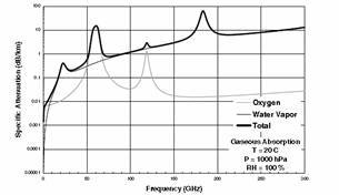
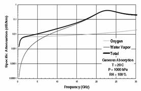
Figure 1. Clear air specific attenuation vs. frequency in the Figure 2. Clear air specific attenuation vs. UHF, SHF, and EHF bands. frequency in the UHF and SHF bands.
Clouds and fog
Scattering by the very small liquid water droplets that make up liquid water fogs near the Earths surface and liquid water clouds higher in the atmosphere can produce significant attenuation at the higher frequencies. Typical liquid water contents range from 0.003 to 3 g/m3 depending on location, height in the atmosphere, and meteorological conditions. Clouds in the most active parts of mid-latitude thunderstorms may have liquid water contents in excess of 5 g/m3. The liquid water cloud heights in the atmosphere can range from 0 km above ground (a fog) to 6 km above ground in the strong updrafts in convective clouds. For a 1-5 g/m3 cloud at a water temperature of 10C, the specific attenuation increases monotonically with frequency through the UHF, SHF, and EHF frequency bands. For frequencies lower than 10 GHz, cloud (or fog) attenuation can be ignored. At a frequency of 30 GHz, cloud attenuations on a 50 elevation angle path may approach 3 to 4 dB. At a frequency of 120 GHz, this result translates to 30 to 40 dB.
Loss from moisture and precipitation
Moisture in the atmosphere takes many forms, some of which play a significant role in attenuating electromagnetic waves. The effects are, of course, frequency-dependent. Precipitation in the form of rain, freezing rain, or wet snow is a significant problem above about 10 GHz. Dry snow and dust also presents a unique challenge to the modeler.
Building material
In practice a signal is normally passing from free-space
through a material like a wall and back into free-space where the receiver is
located. For typical walls, the construction is usually not a single
homogeneous material with well-known properties. A typical
The specific attenuation values for the building materials in Table 2 are significantly lower than the values for water. Water contained in wood or as a mixture in any other material (such as wet sand) increases the specific attenuation. Both concrete and glass produce significantly higher specific attenuation values in the EHF band.
Table 2. Dielectric Properties of Building Materials
|
Frequency(GHz) |
Material |
Dielectric constant |
Loss tangent |
Specific attenuation (dB/m) |
|
Concrete | ||||
|
Fiberglass | ||||
|
Glass | ||||
|
Lightweight concrete | ||||
|
Concrete (dry) | ||||
|
| ||||
|
Teflon | ||||
|
Wood | ||||
|
Concrete | ||||
|
Glass | ||||
|
Concrete |
The elements of building structures the walls, floors, and roofs are generally constructed from several different materials, each with its own dielectric and conductivity properties. Electromagnetic waves are scattered by, reflected from, and transmitted through buildings. Buildings have openings such as windows and doors that have transmission properties different from the surrounding walls. The calculation of the scattered fields is complex. Measurements have been made to characterize the scattering properties of typical buildings. Such measurements have been made by many researchers for cellular and personal communication service (PCS) frequencies below 2 GHz. For fixed broadband wireless systems currently being designed, the bands from 2 to 2.7 GHz. 3.5 to 2.7 GHz. and 5.1 to 5.8 GHz are of primary importance. Unlike cellular frequencies, there is relatively little published data for building penetration losses for these frequencies.
Vegetation
Leaves and branches of individual trees scatter electromagnetic waves. Measurements show differences in the path loss through a tree with season and, at higher frequencies, with the amount of water in and on the leaves. Path loss also depends on the number and species of trees along the path and the height and orientation of the propagation path through the trees. For NLOS Point-to-Multipoint (PMP) systems trees and other foliage will very likely be present on a wireless transmission. Consequently, for residential, small office buildings, and other low profile structures where trees may extend above the height of the receiver antenna location, the attenuation or path loss due to foliage must be considered along with building penetration loss.
Obstacles
Obstacles such as buildings, trees, Earth mounds, and hills may attenuate the electromagnetic waves. If the attenuation through the obstacle is high enough, the obstacle will diffract the wave over or around the obstruction. A single propagation path between a transmitting antenna and a receiving antenna is a clear line-of-sight path if no obstructions occur within the first few Fresnel zones about the path. Fresnel zones are enclosed within equiphase ellipsoids enclosing the path. [3], [4], [6], [7]
3.2 Atmospheric Refraction
Refractive and scattering effects of the atmosphere include:
Refraction on horizontal paths resulting in alteration of the radio horizon due to ray curvature.
Troposcatter, from localized fluctuations in the atmospheric refractive index, which can scatter electromagnetic waves.
Temperature inversion, abrupt changes in the refractive index with height causing reflection.
Ducting, where the refractive index is such that electromagnetic waves tend to follow the curvature of the earth.
These effects vary widely with altitude, geographic location, and weather conditions. The effects can permit beyond-the-horizon communication (or interference), or produce blockage and diffraction from terrain that appears to be below the line of sight and multipath fading. Gradual changes in the refractive index with height cause EM waves to bend in the atmosphere. If the atmosphere were homogeneous, the waves (rays) would travel in a straight line and the physical and RF horizons would coincide. The rate of change of the refractive index with height can be approximated as being constant in the first kilometer above sea level. This increases the apparent distance to the horizon, by bending the nearly horizontal rays downward. This is illustrated in Figure 3, where a horizontal ray is bent downward and sees a radio horizon that is beyond the straight line-of-sight horizon (h is the antenna height). By replacing the model of the earths surface with one that has a radius of 4/3 of the earths radius (for a standard reference atmosphere), the curved ray becomes straight. The 4/3 earth radius approximation is derived based on a standard atmosphere at sea level and is therefore not universally applicable. Nonetheless, it is very widely used and often treated as if it were universal.
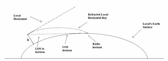
Figure 3 Effect of atmospheric refraction on the distance to the horizon.
It is interesting to note that the ray that reaches the radio horizon is not the same ray that is directed at the LOS horizon, it leaves the source at a slightly greater elevation angle. In the case of very narrow beamwidth antennas, it is possible that the departure angle of the radio horizon ray is outside of the beamwidth of the antenna. If this occurs, then the effect of the refraction can be a reduction in communication distance rather than an increase since the ray leaving the source at the center of the antenna beamwidth will be bent toward the ground and the peak of the transmitted signal will not be directed at the intended receiver. The energy that reaches the receiver will be a combination of off-axis radiation from the antenna and any diffraction from intervening terrain that blocks the bore-sight radiation. For this reason, it is important to verify antenna aiming at different times over a period of days . If aiming is only done once and happens to be done during a period of significant refraction, then under nominal conditions the link margin will be below the design level, reducing the link margin and availability.
Ducting occurs when the curvature of the refraction is identical (or nearly identical) to the curvature of the earth. Another way to look at it is that under ducting conditions, the equivalent earth radius is infinite. There are two primary types of ducts: surface ducts, where the wave is trapped between the earths surface and an inversion layer, and elevated ducts, where the layers of the atmosphere trap the wave from both above and below. Elevated ducts may occur up to about 1500 m above the surface. In either case, both ends of the communication link must be located within the same duct for a signal enhancement to be observed. The case of surface ducting is more common and usually of much greater practical concern. Ducting tends to be primarily an effect due to water vapor content, but it can also be caused by a mass of warm air moving in over cooler ground or the sea or by night frost. [3], [4], [7]
4. Model Classifications
Given the significance of propagation and channel models in designing and building successful communication systems, a considerable amount of effort has been devoted by the industry to developing such models. Thus, propagation and channel models will be divided into three basic classifications:
Theoretical
Empirical
Physical
These model classifications will be discussed in more detail later with some specific examples. Theoretical models have relatively little application to fixed broadband wireless systems except as they may be applied to predict rain attenuation. Empirical models are based on measurement or observations of signal performance in real propagation environments. Their use for dimensioning non-line-of-sight (NLOS) point-to-multipoint systems is becoming more widespread. Physical models make use of the physical mechanisms of electromagnetic (EM) wave propagation to predict signal attenuation and channel response. Such models are the most widely used for fixed broadband wireless systems. Physical models are sometimes described as deterministic models; a term borrowed from probability analysis that is more appropriately applied to channel modeling in which the channel response characteristics may be divided between deterministic and random processes. [4]
It is often argued that results from deterministic electromagnetic-based calculation models are not expressed in terms of parameters that can be used in the simulation of wireless communications systems. Parameters such as delay spread, coverage, direction of arrival, and bit error rate (BER) are necessary for system simulations and need to be incorporated as part of the simulation code development.
Four different types of methods are often used in developing propagation models, and the above listed limitations are expected to impact them differently. For example, statistical models provide parameters suitable for system simulations but lack specificity and accuracy. EM-based deterministic models, on the other hand, provide accurate and site specific coverage and delay spread information but are also very computationally inefficient and time consuming. Empirical and measurement-based models are site specific, frequency specific, and hence lack generality. Researchers use a combination of these methods to help improve the accuracy, broaden the generality, and reduce the required computational time. But much more research and development are needed to fully develop accurate, computationally efficient, and experimentally verified propagation models that may be used for broadband and highly mobile communications systems. With the advances in the signal processing methods and the development of communications algorithms, the envisioned propagation models are expected to play a critical role in the accurate accounting for mobility and the dynamic variation in the characteristics of the propagation channels. [2]
Channel models are often classified as narrowband or wideband. A narrowband model is one based on the predicted mean signal level and some assumptions about the signal envelope fading statistics around this predicted mean level. The assumption is that because of the limited bandwidth of the signal being sent through the channel, more detailed information is not required to provide a useful prediction of the channel effect on the signal. Because the signal bandwidth is narrow, the fading mechanism will affect all frequencies in the signal passband equally. For this reason, a narrowband channel is often referred to as a flat-fading channel.
For wideband channel models, the assumption is that the bandwidth of the signal sent through the channel is such that time dispersion information, in addition to mean signal level information, is required. Time dispersion causes the signal fading to vary as a function of frequency, so wideband channels are often called frequency selective fading channels.
This outline defines channel models in terms of how they work and the information they provide, rather than the bandwidth of the signal that can successfully be used with them. The three main model categories are theoretical, empirical, and physical, with non-time-dispersive and time dispersive models as the primary subcategories. A time-dispersive model is one designed to provide information about the time delay experienced by a transmitted signal and its multipath replicas in reaching the receiver.
Classification of propagation/channel models.
Physical
Theoretical Empirical
4.1 Theoretical Models
Models in this category are based on some theoretical assumptions about the propagation environment. They do not directly use information about any specific environment, although the assumptions may be based on measurement data or physical laws. Theoretical models are useful for analytical studies of the behavior of communication systems under a wide variety of channel response circumstances, but because they do not deal with any specific propagation information, they are not suitable for planning communication systems to serve a particular area. With this objective, they usually rely on assumptions that lead to mathematically tractable formulations.
Non time-dispersive
The classic channel models by
Time-dispersive
Examples of theoretical time-dispersive models are those
of
4.2 Empirical Models
In the VHF/UHF frequency bands, a classic example of an
empirical propagation model is the Federal Communications Commission (FCC)
model. The FCC model is actually composed of equations that were fitted to a
set of signal strength measurements done at several locations in the
Empirical models fundamentally use experimental measurement data to deduce a relationship between the propagation circumstances and expected field strength or time dispersion results. Because they use statistical specifiers that have no direct physical relationship to the quantity being predicted, they are inherently non-causal. They are also inherently not site-specific since they do not explicitly take into account the unique features of a given propagation environment along a path from a transmitter to a receiver.
Non time-dispersive
For the non-time-dispersive case, there are a large number of models that have been developed over the years. The FCC, ITU-R, and Hata models mentioned earlier are examples of empirical propagation models. There are several others, including Egli, EdwardDurkin, BlomquistLadell, and AllsebrookParsons. All of these models use some measurement sets and a statistical analysis of the data to construct a curve through the data. The objective is to simply predict mean path loss as a function of antenna heights, height above average terrain, terrain roughness, or other parameters such as local clutter (foliage and buildings). The AllsebrookParsons model is interesting in that it attempts to predict path loss in urban areas using the orientation and widths of streets.
Time-dispersive
Empirical models that provide time dispersion information
are rare. Like predicting mean path loss based on a measurement set, a
corresponding time dispersion model would use measured time delay profiles from
which statistically derived curves, or simple look-up tables, yield a way of
predicting time dispersion in some given environment based on its characteristics.
Models in this classification were developed by the
4.3 Physical Models
As pointed out earlier, physical models rely on the basic principles of physics rather than statistical outcomes from experiments to find the EM field at a point. Physical models are causal by design. Depending on whether they consider the particular elements of the propagation environment between a transmitter and receiver, physical models may or may not be site-specific. Also, they may or may not provide time dispersion information. One aspect that affects the capabilities and success of a physical model is the kind of information about the propagation environment it can use and what it does with it. This is an important point about physical propagation modeling. The quality of the models predictions is a direct consequence of how the model maps the real propagation environment into the model propagation environment. For a channel model to be a physical, site-specific model, it not only must use the physical laws of EM wave propagation but it must also have a systematic technique for mapping the real propagation environment into the model propagation environment.
Non time-dispersive and not site-specific
A physical, not site-specific model uses physical principles of EM wave propagation to predict signal levels in a generic environment in order to develop some simple relationships between the characteristics of that environment and propagation. An apt example of this approach is the WalfischIkegami model for mobile radio systems in urban areas where roof edges are considered as a series of diffracting screens with a final edge diffraction from building roof to the street level being included.
Non time-dispersive and site-specific
A physical, not time-dispersive model is one in which the
EM field at the receiver is predicted using physical laws governing wave
propagation, but no signal time delay information is available from the model. Models
in this category include a collection of propagation algorithms to predict
signal attenuation over terrain. An early example is by Bullington who actually
prepared nomographs to make his model more directly useful to practicing
engineers. Other examples of models are the LongleyRice, TIREM, Free Space+RMD,
and the
Time-dispersive and site-specific
These models are basically known as ray-tracing, a
high-frequency approximation method that tracks the trajectory of EM waves
leaving the transmitter as they interact with objects in the propagation
environment. Since a ray-tracing model tracks ray trajectories, it not only
provides time dispersion information but also angle-of-arrival information that
is of great interest in assessing the operation of adaptive or smart
antennas. Interestingly, perhaps the earliest example of ray-tracing models
comes from broadcasting rather than from the mobile radio. The NTSC television
signal used in the
broadcast signals are by Ikegami and his coworkers. [2], [4]
5. Near-Earth Propagation Models
These models are all based on measurements (sometimes with theoretical extensions) and represent a statistical mean or median of the expected path loss. Much of the data collection for near-earth propagation impairment has been done in support of mobile VHF communications and, more recently, mobile telephony (which operates between 800MHz and 2GHz). Thus many of the models are focused in this frequency range. While for the most part, models based on this data are only validated up to 2GHz, in practice they can sometimes be extended beyond that if required.
5.1 Foliage Models
Most terrestrial communications systems require signals to pass over or through foliage at some point. This section presents a few of the better-known foliage models. These models provide an estimate of the additional attenuation due to foliage that is within the line-of-sight (LOS) path. There are of course, a variety of different models and a wide variation in foliage types. For that reason, it is valuable to verify a particular models applicability to a given region based on historical use or comparison of the model predictions to measured results.
Weissbergers Model
Weissbergers modified exponential decay model is given by
where
df is the depth of foliage along the LOS path in meters
F is the frequency in GHz
The attenuation predicted by Weissbergers model is in addition to free-space (and any other nonfoliage) loss. Weissbergers modified exponential decay model applies when the propagation path is blocked by dense, dry, leafed trees. It is important that the foliage depth be expressed in meters and that the frequency is in GHz. Blaunstein indicates that the model covers the frequency range from 230MHz to 95GHz.
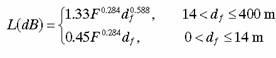
Early ITU Vegetation Model
The early ITU foliage model was adopted by the CCIR (the ITUs predecessor) in 1986.While the model has been superseded by a more recent ITU recommendation, it is an easily applied model that provides results that are fairly consistent with the Weissberger model. The model is given by
![]()
where
F is the frequency in MHz
df is the depth of the foliage along the LOS path in meters
Updated ITU Vegetation Model
The current ITU models are fairly specific and do not cover all possible scenarios. Nonetheless they are valuable and represent a recent consensus. One of the key elements of the updated model, which should also be considered in applying other models is that there is a limit to the magnitude of the attenuation due to foliage, since there will always be a diffraction path over and/or around the vegetation.
5.2 Terrain Modeling
For ground-based communications, the local terrain features significantly affect the propagation of electromagnetic waves. Terrain is defined as the natural geographic features of the land over which the propagation is taking place. It does not include vegetation or man-made features. When the terrain is very flat, only potential multipath reflections and earth diffraction, if near the radio horizon, need to be considered. Varied terrain, on the other hand, can produce diffraction loss, shadowing, blockage, and diffuse multipath, even over moderate distances. The purpose of a terrain model is to provide a measure of the median path loss as a function of distance and terrain roughness. The variation about the median due to other effects are then treated separately.
Egli Model
While not a universal model, the Egli models ease of implementation and agreement with empirical data make it a popular choice, particularly for a first analysis. The Egli model for median path loss over irregular terrain is
![]()
where
Gb is the gain of the base antenna
Gm is the gain of the mobile antenna
hb is the height of the base antenna
hm is the height of the mobile antenna
d is the propagation distance
β = (40/f )2, where f is in MHz
Note that the Egli model provides the entire path loss, whereas the foliage models discussed earlier provided the loss in addition to free-space loss. Also note that the Egli model is for irregular terrain and does not address vegetation. While similar to the ground-bounce loss formula, the Egli model is not based on the same physics, but rather is an empirical match to measured data. By assuming a log-normal distribution of terrain height, Egli generated a family of curves showing the terrain factor or adjustment to the median path loss for the desired fade probability. This way the analyst can determine the mean or median signal level at a given percentage of locations on the circle of radius d. Stated another way, the Egli model provides the median path loss due to terrain loss.
LongleyRice Model
The LongleyRice model is a very detailed model that was developed in the 1960s and has been refined over the years. The model is based on data collected between 40MHz and 100GHz, at ranges from 1 to 2000km, at antenna heights between 0.5 and 3000m, and for both vertical and horizontal polarization. The model accounts for terrain, climate, and subsoil conditions and ground curvature. Because of the level of detail in the model, it is generally applied in the form of a computer program that accepts the required parameters and computes the expected path loss. As indicated in the previous section, the LongleyRice model has two modes, point-to-point and area. The point-to-point mode makes use of detailed terrain data or characteristics to predict the path loss, whereas the area mode uses general information about the terrain characteristics to predict the path loss.
5.3 Propagation in Built-Up Areas
Propagation of electromagnetic waves through developed areas from suburban to dense urban is of considerable interest, particularly for mobile telephony. This is a vast subject with numerous papers and models available. The actual propagation of RF though an urban environment is dependent upon frequency, polarization, building geometry, material structure, orientation, height, and density. This section treats propagation between elevated base stations and mobiles that are at street level in urban and suburban areas. The goal is to determine the median path loss or RSL as a function of the distance, d, so that the required multipath fading models can then be applied. The median value depends heavily upon the size and density of the buildings, so classification of urban terrain is important. The models discussed are the Young, Okumura, Hata, and Lee models.
Young Model
The
Young data were taken in
![]()
where β is called the clutter factor and is not the same β used in the Egli model! This β is also distinct from the β sometimes used for building volume over a sample area in classification.
Okumura Model
The
Okumura model is based on measurements made in
correction factors applied for some parameters. For the Okumura model, the prediction area is divided into terrain categories: open area, suburban area, and urban area. The open-area model represents locations with open space, no tall trees or buildings in the path, and the land cleared for 300400 m ahead (i.e., farmland). The suburban area model represents a village or a highway scattered with trees and houses, some obstacles near the mobile, but not very congested. The urban area model represents a built-up city or large town with large buildings and houses with two or more stories, or larger villages with close houses and tall thickly grown trees. The Okumura model uses the urban area as a baseline and then applies correction factors for conversion to other classifications. A series of terrain types is also defined. Quasi-smooth terrain is the reference terrain and correction
factors are applied for other types of terrain. Okumuras expression for the median path loss is
![]()
where
LFSL is the free-space loss for the given distance and frequency
Amu is the median attenuation relative to free-space loss in an urban area, with quasi-smooth terrain; the value of Amu is a function of both frequency and distance
hte = 200m is the base station effective height
hre = 3m is the mobile antenna height
Htu is the base station height gain factor
Hru is the mobile antenna height gain factor
Hata Model
The Hata model (sometimes called the OkumuraHata model) is an empirical formulation that incorporates the graphical information from the Okumura model. There are three different formulas for the Hata model:
Urban Areas
![]()
where
150 < fc < 1500, fc in MHz
30 < ht < 200, ht in m
1 < d < 20, d in km
and a(hr) is the mobile antenna height correction factor.
For a small or medium-sized city:
![]()
and for a large city:
![]()
Suburban Areas
![]()
Open Areas
![]()
Lee Model
The Lee model was originally developed for use at 900MHz and has two modes: area-to-area and point-to-point. Even though the original data are somewhat restrictive in its frequency range, the straightforward implementation, ability to be fitted to empirical data, and the results it provides make it an attractive option. The model includes a frequency adjustment factor that can be used to increase the frequency range analytically. The Lee model is a modified power law model with correction factors for antenna heights and frequency. A typical application involves taking measurements of the path loss in the target region and then adjusting the Lee model parameters to fit the model to the measured data.
Lee Area-to-Area Mode. For area-to-area prediction, Lee uses a reference median path loss at one mile, called L0, the slope of the path loss curve, λ in dB/decade, and an adjustment factor F0. The median loss at distance, d, is given by
![]()
Lees model was originally formulated as a received signal level prediction based on a known transmit power level and antenna gains. The formulation presented here has been converted from an RSL model to a path loss model to better fit the format of the other models presented.
Lee Point-to-Point Mode. The point-to-point mode of the Lee model includes an adjustment for terrain slope. The median path loss is given by
![]()
or
![]()
where heff is in meters; heff is determined by extrapolating the terrain slope at the mobile back to the base station antenna and then computing the antenna height (vertically) above the extrapolated line. [3], [7], [8]
6. Indoor Propagation Modeling
Indoor propagation of electromagnetic waves is central to the operation of wireless LANs, cordless phones, and any other indoor systems that rely on RF communications. The indoor environment is considerably different from the typical outdoor environment and in many ways is more hostile. Modeling indoor propagation is complicated by the large variability in building layout and construction materials. In addition, the environment can change radically by the simple movement of people, closing of doors, and so on. For these reasons, deterministic models are not often used. In this chapter, some statistical (site-general) models are presented. When fit to empirical data, these models can provide a reasonable representation of the indoor environment.
6.1 Interference
While an understanding of indoor propagation is essential, another important element of indoor wireless operation that should be considered is interference. Unlike outdoor environments, where the operating distances are greater, in an indoor environment, it is possible, and in fact common, to have an interfering system operating within a few feet or less of a given system. A classic but by no means isolated example is the desktop computer with a wireless LAN card that also employs a wireless keyboard and/or mouse. The wireless keyboard and mouse are likely to use the Bluetooth standard, which uses frequency hopping in the 2.4-GHz ISM band. If the wireless LAN card is an 802.11b or g [direct sequence spread spectrum (DSSS) or orthogonal frequency division multiplexing (OFDM)] system, then it will be operating in the same frequency band and the potential for interference exists. In addition, a computer has a variety of internal high-frequency digital clocks that generate harmonics, which may fall within the systems passband. A monitor may also produce a substantial amount of interference. Add to that the RF energy radiated by fluorescent lighting, other consumer products, and office equipment, and it becomes clear that the interference environment indoors is very unfriendly. It is important to account for this interference and to understand that communication link problems in indoor environments may not be propagation issues, but rather interference issues. Sometimes simply repositioning a piece of equipment by a few feet is enough to resolve the problem.
6.2 The Indoor Environment
The principal characteristics of an indoor RF propagation environment that distinguish it from an outdoor environment are that the multipath is usually severe, a line-of-sight path may not exist, and the characteristics of the environment can change drastically over a very short time or distance. The ranges involved tend to be rather short, on the order of 100 m or less .Walls, doors, furniture, and people can cause significant signal loss. Indoor path loss can change dramatically with either time or position, because of the amount of multipath present and the movement of people, equipment, and/or doors.
6.2.1 Indoor Propagation Effects
When considering an indoor propagation channel, it is apparent that in many cases there is no direct line of sight between the transmitter and receiver. In such cases, propagation depends upon reflection, diffraction, penetration, and, to a lesser extent, scattering. In addition to fading, these effects, individually and in concert, can degrade a signal. Delay and Doppler spread are usually far less significant in an indoor environment because of the much smaller distances and lower speeds of portable transceiver as compared to outdoor environments. However, this advantage is usually offset by the fact that many indoor applications are wideband, having short symbol times and therefore a corresponding greater sensitivity to delay spread. In addition, the wave may experience depolarization, which will result in polarization loss at the receiver.
6.2.2 Indoor Propagation Modeling
There are two general types of propagation modeling: site-specific and site-general. Site-specific modeling requires detailed information on building layout, furniture, and transceiver locations. It is performed using ray-tracing methods in a CAD program. For large-scale static environments, this approach may be viable. For most environments however, the knowledge of the building layout and materials is limited and the environment itself can change, by simply moving furniture or doors. Thus the site-specific technique is not commonly employed. Site-general models provide gross statistical predictions of path loss for link design and are useful tools for performing initial design and layout of indoor wireless systems. Two popular models, the ITU and the log-distance path loss models, are discussed in the following sections.
6.2.3 The ITU Indoor Path Loss Model
The ITU model for site-general indoor propagation path loss prediction is
![]()
where
N is the distance power loss coefficient
f is the frequency in MHz
d is the distance in meters (d > 1m)
Lf(n) is the floor penetration loss factor
n is the number of floors between the transmitter and the receiver
Table 3. Representative values for the power loss coefficient, N, as given by the ITU
|
Frequency |
Residential |
Office |
Commercial |
|
900MHz | |||
|
1.21.3GHz | |||
|
1.82GHz | |||
|
4GHz | |||
|
5.2GHz | |||
|
60GHz |
A power loss coefficient value of N = 20 corresponds to free-space loss, and this will usually apply in open areas. Corridors may channel RF energy, resulting in a power loss coefficient of N = 18 (slightly less than free-space loss). In the case of propagation around corners or through walls, N = 40 is used. For long paths, the reflected path(s) may interfere, resulting in N = 40 being used here as well.
6.2.4 The Log-Distance Path Loss Model
The log-distance path loss model is another site-general model and it is given by
![]()
where
PL(d0) is the path loss at the reference distance, usually taken as (theoretical) free-space loss at 1m
d/d0 is the path loss distance exponent
Xs is a Gaussian random variable with zero mean and standard deviation of δ dB
Other indoor propagation models include the Ericsson multiple breakpoint model, which provides an empirical worst-case attenuation versus distance curve, and the attenuation factor model, which is similar in form to the log-distance model. There are a variety of empirical models for indoor propagation loss, most of which are modified power law. Any model used should either be optimized for the particular application if possible, or otherwise, additional margin included in the design. Empirical path loss prediction models should be used to determine a high level design. Once the design is complete, field measurements or an actual deployment serve as the final determination of a models applicability to a given building. A good static design must still include sufficient margin for the environmental dynamics. Depending upon the bandwidth and data rate, delay spread effects may also need to be considered. As a rule, the delay spread
effects are considered by the modem or equipment designer and not by the individual who lays out the network, since the mitigation is best handled at the equipment level.
7. Conclusions/ Disscusions
With the phenomenal growth in mobile and portable terrestrial wireless communication systems, and due to their potential utilization in a wide variety of high data rate and multimedia services, higher frequency bands need to be allocated and utilized for these services. New devices and components for high frequency and millimeter wave integrated front-end receivers are being developed, active and low cost phased array antennas are being designed, and advanced software issues in coding, modulation, switching, and networking are being researched and developed. In addition to these rather obvious advances that are needed to enable the next generation wireless technology, developing new and more computationally efficient propagation models is also essential. Development of reliable propagation models and the availability of the associated simulation software tools would be absolutely necessary for the successful implementation of the future terrestrial wireless systems and also for their integration with other technologies including the satellite, LMDS (local multi-point distribution systems), and the wireline based services. Accurate propagation models will help in using the rather congested frequency spectrum more efficiently, in planning more effective radio networks, and in implementing cost effective solutions for a desirable and user specific communication coverage pattern. [2]
The goal of propagation modeling is often to determine the probability of satisfactory performance of a communication system or other system that is dependent upon electromagnetic wave propagation. It is a major factor in communication network planning. If the modeling is too conservative, excessive costs may be incurred, whereas too liberal of modeling can result in unsatisfactory performance. Thus the fidelity of the modeling must fit the intended application. [3]
8. References/ External Links
[1]. Radio Propagation Models https://people.seas.harvard.edu/~jones/es151/prop_models/propagation.html#propmain
[2]. CHANNEL CHARACTERIZATION AND PROPAGATION MODELS FOR WIRELESS COMMUNICATION SYSTEMS
https://www.wtec.org/loyola/wireless/04_01.htm
Introduction to RF Propagation by John S. Seybold
[4]. Fixed Broadband Wireless System Design - by Harry R. Anderson
https://books.google.ro/books?id=M8NOGnp2IRwC&printsec=frontcover
[5]. L1_General concepts on propagation Laboratory 1 from Antennas & Propagation Course
[6]. L2_Basic concepts on wireless systems - Laboratory 2 from Antennas & Propagation Course
[7]. Propagation Handbook for Wireless Communication System Design by Robert K. Crane
[8]. L4_Models to Predict Propagation Losses - Laboratory 1 from Antennas & Propagation Course
[9]. https://en.wikipedia.org/wiki/Ray_tracing_(physics)
|
Politica de confidentialitate | Termeni si conditii de utilizare |

Vizualizari: 3630
Importanta: ![]()
Termeni si conditii de utilizare | Contact
© SCRIGROUP 2026 . All rights reserved