| CATEGORII DOCUMENTE |
| Bulgara | Ceha slovaca | Croata | Engleza | Estona | Finlandeza | Franceza |
| Germana | Italiana | Letona | Lituaniana | Maghiara | Olandeza | Poloneza |
| Sarba | Slovena | Spaniola | Suedeza | Turca | Ucraineana |
Introduction
As discussed in Lecture 2, the general three-dimensional state of stress is obtained, as was discussed in Lecture 2, by passing a set of three orthogonal planes though a point of the solid body and isolating the infinitesimal volume located around the point. The three-dimensional state of stress is illustrated in Figure 1 where, for clarity, only the stresses drawn on the faces with positive normal are represented.
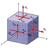
Figure 1 Three-Dimensional State of Stress
Mathematically the three-dimensional state of stress is
represented by a generalized stress tensor![]() defined by nine distinct stress components:
defined by nine distinct stress components:
 (1)
(1)
Applying the shear stress duality principle the number of independent tensorial components is reduced from nine to six and, consequently, the symmetric shear stress components are related as:
![]() (2)
(2)
![]() (3)
(3)
![]() (4)
(4)
There are instances when some of the stress tensor
components vanish and the general three-dimensional stress tensor ![]() degenerates into a tensor characterized by only three
independent components. This condition is called plane state of stress. For the present theoretical development, it
is assumed that all stress components pertinent to the planes having normal
vector parallel to the
degenerates into a tensor characterized by only three
independent components. This condition is called plane state of stress. For the present theoretical development, it
is assumed that all stress components pertinent to the planes having normal
vector parallel to the ![]() axis are zero:
axis are zero:
![]() (5)
(5)
![]() (6)
(6)
![]() (7)
(7)
This type of plane stress tensor is illustrated in Figure 2.
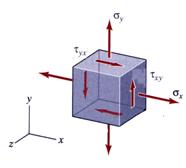
Figure 2 Plane Stress Tensor
Additionally, the remaining non-zero stress tensor
components contained in equation (1) are assumed to be independent of the
variable![]() .
.
![]() (8)
(8)
Consequently, the plane stress tensor ![]() can be represented in
plane
can be represented in
plane![]() as depicted in Figure 3:
as depicted in Figure 3:
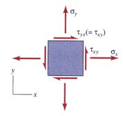
Figure 3
The plane stress tensor![]() is defined by three non-zero components:
is defined by three non-zero components:
 (9)
(9)
Several of the conditions encountered in previous lectures, including the study of the axial and torsional deformation and pure and non-uniform bending, are characterized by different states of plane stress. In reality, the plane stress tensor is a direct result of the assumptions imposed on the deformation.
Examples of plane stress tensors, such as uni-axial, pure shear and bi-axial, are illustrated in Figure 4.
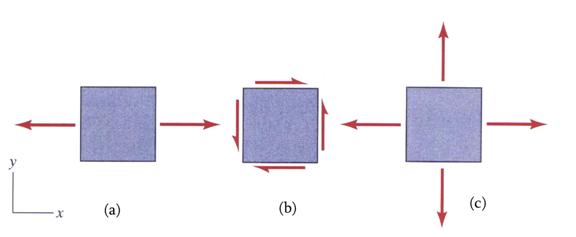
Figure 4 Examples of
(a) Uni-Axial, (b) Pure Shear and (c) Bi-Axial
Plane Stress Transformation Equations
Suppose that the components of the plane stress tensor![]() , as expressed by equation (9), are defined at any point
, as expressed by equation (9), are defined at any point ![]() of the vertical plane
of the vertical plane![]() . The variation of stress components when the reference
system attached to point
. The variation of stress components when the reference
system attached to point ![]() is rotated with a
counterclockwise angle
is rotated with a
counterclockwise angle ![]() , as illustrated in Figure 5, is the subject of this section.
, as illustrated in Figure 5, is the subject of this section.
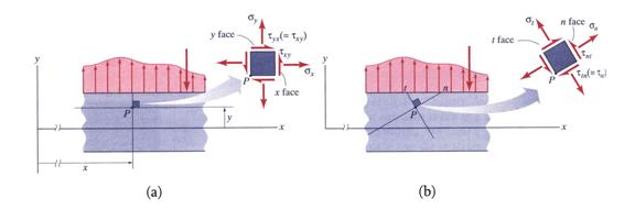
Figure 5 Representation of the
(a) Normal Planes and (b) Rotated Planes
The transformation relations between stresses ![]() ,
, ![]() and
and![]() pertinent to a rotated plane and the stresses
pertinent to a rotated plane and the stresses![]() ,
, ![]() and
and ![]() are obtained by
writing the equilibrium equations for the infinitesimal triangular element depicted
in Figure 6. The inclined plane is defined by its positive normal
are obtained by
writing the equilibrium equations for the infinitesimal triangular element depicted
in Figure 6. The inclined plane is defined by its positive normal ![]() which is rotated counterclockwise with an angle
which is rotated counterclockwise with an angle![]() from the horizontal direction
from the horizontal direction ![]() .
.
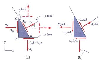
Figure 6 Equilibrium of the Infinitesimal Triangular Element
(a) Stresses and (b) Forces
Using the notation shown in Figure 6.b the equilibrium equations are written as:
![]()
 (10)
(10)
![]()
 (11)
(11)
From Figure 6 the following geometrical relations can be derived:
![]() (12)
(12)
![]() (13)
(13)
Substituting equations (12) and (13)
into equations (10) and (11) and using the shear stress duality principle the
following expressions are obtained for normal![]() and shear
and shear![]() stresses:
stresses:
![]() (14)
(14)
![]() (15)
(15)
Equations (14) and (15) can be re-written using the trigonometric
relations between the angle![]() and the double angle
and the double angle![]() :
:
![]() (16)
(16)
![]() (17)
(17)
Equation (16) and (17) are called the plane stress transformation equations.
In general, two faces are needed to express the plane stress
tensor around a point ![]() . Consequently, the formulae (16) and (17) are applied twice:
first, considering the rotation angle
. Consequently, the formulae (16) and (17) are applied twice:
first, considering the rotation angle ![]() and, secondly, for the
complementary angle
and, secondly, for the
complementary angle![]() . The notation is illustrated in Figure 7. The rotation
angles
. The notation is illustrated in Figure 7. The rotation
angles ![]() and
and ![]() are related as:
are related as:
![]() (18)
(18)
The relation between the double angles necessary in equations (16) and (17) is obtained as:
![]() (19)
(19)
Consequently, the following trigonometric relations can be established:
![]() (20)
(20)
![]() (21)
(21)
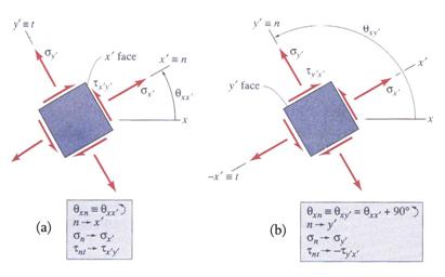
Figure 7 Stresses on Orthogonal Rotated Faces
The stresses on two orthogonal rotated faces are expressed as:
 (22)
(22)
 (23)
(23)
 (24)
(24)
 (25)
(25)
If equations (22) and (24) are summed, the invariance of the summation of normal stresses is established:
![]() (26)
(26)
Principal Stresses
The maximum and minimum normal stresses are called principal stresses and mathematically
represent the extreme values of the normal stress function ![]() . The extreme values are obtained by imposing the condition that
the first derivative of the normal stress
. The extreme values are obtained by imposing the condition that
the first derivative of the normal stress ![]() relative to the
rotation angle
relative to the
rotation angle ![]() is zero:
is zero:
![]() (27)
(27)
The explicit expression for equation (27) is obtained by differentiating equation (16):
![]() (28)
(28)
Dividing by 2*![]() the trigonometric equation (28) is transformed into equation
(29) relating the tangent of twice the principal directions angle,
the trigonometric equation (28) is transformed into equation
(29) relating the tangent of twice the principal directions angle, ![]() , to the stresses ion the orthogonal planes
, to the stresses ion the orthogonal planes ![]() and
and ![]() :
:
 (29)
(29)
The angle ![]() represents the angle for which the normal stress
represents the angle for which the normal stress![]() reaches its extreme value. The geometrical illustration of
the equation (29) is presented in Figure 8.a where the distance
reaches its extreme value. The geometrical illustration of
the equation (29) is presented in Figure 8.a where the distance![]() is calculated as:
is calculated as:
 (30)
(30)
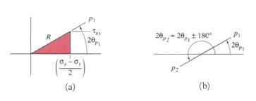
Figure 8 Geometrical Representation of Equation (29)
Solution of the trigonometric equation (29) yields two
solutions, ![]() and
and![]() , where the two angles are related as:
, where the two angles are related as:
![]() (31)
(31)
From equation (31), the orthogonality of the two principal directions is established:
![]() (32)
(32)
To calculate the values of the normal stress ![]() corresponding to the angles
corresponding to the angles ![]() and
and ![]() it is necessary to
evaluate the trigonometric functions
it is necessary to
evaluate the trigonometric functions ![]() and
and ![]() contained in equation
(16). Using the notation shown in Figure 8.a and the trigonometric relations (20)
and (21) these functions can be expressed as:
contained in equation
(16). Using the notation shown in Figure 8.a and the trigonometric relations (20)
and (21) these functions can be expressed as:
![]() (33)
(33)
 (34)
(34)
![]() (35)
(35)
 (36)
(36)
Substituting first the trigonometric expressions (33) and (34)
into equation (16) and then (35) and (36) the principal stresses ![]() and
and ![]() are obtained:
are obtained:
 (37)
(37)
 (38)
(38)
The average normal stress is calculated as:
![]() (39)
(39)
The principal stresses are schematically depicted in Figure 9.
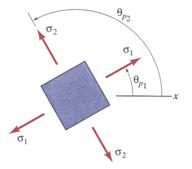
Figure 9 Principal Stresses and Directions
The right-hand expression of equation (28) being identical with
the expression (17), representing the shear stress![]() , allows equation (28) to be re-written as:
, allows equation (28) to be re-written as:
![]() (40)
(40)
Equation (40) indicates that the principal normal stresses are obtained for a rotated plane where the shear stress is zero.
The invariance of the sum of the normal stresses is again shown to be valid for the case of the principal stresses. Summation of equations (37) and (38) yields:
![]() (41)
(41)
To identify which of the two angles, ![]() or
or![]() , corresponds to the maximum principal stress
, corresponds to the maximum principal stress ![]() the second derivative
of the function
the second derivative
of the function ![]() relative to the
rotation angle
relative to the
rotation angle ![]() is employed. The
condition for the point to be a maximum is:
is employed. The
condition for the point to be a maximum is:
![]() (42)
(42)
The condition (42) is explicitly written as:
![]() (43)
(43)
The inequality (43) can be manipulated and cast in a new form:
![]() (44)
(44)
If the ![]() is expanded the following trigonometric expression is established:
is expanded the following trigonometric expression is established:
![]() (45)
(45)
Substituting equations (29) and (45), representing the ![]() and
and ![]() , into the inequality (44) the following expression is
obtained:
, into the inequality (44) the following expression is
obtained:
 (46)
(46)
The condition for the inequality (46) to hold true is:
![]() (47)
(47)
Note: It is important to note that for the inequality (47) to hold true,
the signs of the tangent of the angle ![]() and shear stress
and shear stress![]() must be identical.
must be identical.
The angle corresponding to the direction of the maximum normal
stress can also be obtained by successively assigning to the angle ![]() in equation (16) the
values
in equation (16) the
values ![]() and
and ![]() and observing which
angle produces the maximum principal stress.
and observing which
angle produces the maximum principal stress.
Maximum Shear Stresses
The maximum shear stresses are determined in a similar
manner as the principal stresses. The extreme condition for the shear stress
function![]() contained in equation (17) is written as:
contained in equation (17) is written as:
![]() (48)
(48)
The explicit format of equation (48) is obtained by differentiating the expression (17):
![]() (49)
(49)
Dividing by ![]() the trigonometric
equation (49), the tangent of the principal directions angle
the trigonometric
equation (49), the tangent of the principal directions angle ![]() is obtained:
is obtained:
 (50)
(50)
The angle ![]() represents the angle for which the shear stress
represents the angle for which the shear stress![]() reaches its extreme value. Equation (50) is illustrated in
Figure
reaches its extreme value. Equation (50) is illustrated in
Figure
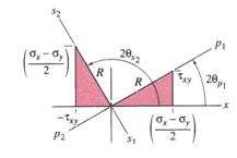
Figure 10 Angular Relation between ![]() and
and ![]()
Solving the trigonometric equation (50), two solutions ![]() and
and![]() are obtained. They are related as:
are obtained. They are related as:
![]() (51)
(51)
Dividing equation (50) by two (2), the orthogonality of the two
angles![]() and
and![]() is obtained:
is obtained:
![]() (52)
(52)
Equation (50) indicates that a relation between the angles ![]() and
and ![]() can be established. With this intent, equation (50) is recast
into a new format as follows:
can be established. With this intent, equation (50) is recast
into a new format as follows:
![]() (53)
(53)
First, multiplying by the terms in the denominator, equation (53) becomes:
![]() (54)
(54)
Then, equation (54) is simplified as:
![]() (55)
(55)
Therefore,
![]() (56)
(56)
The relationship between angles ![]() and
and ![]() is calculated from
equation (56):
is calculated from
equation (56):
![]() (57)
(57)
Still, equation (57) does not indicate how to identify the direction of the maximum shear stress. By examination of Figure 10, the following angular relations can be established:
![]() (58)
(58)
The relationship between the angles of the maxim principal
and shear stress directions, ![]() and
and ![]() , is obtained from (58) as:
, is obtained from (58) as:
![]() (59)
(59)
Again using the notation shown in Figure 10, the following trigonometric relations are obtained:
 (60)
(60)
![]() (61)
(61)
 (62)
(62)
![]() (63)
(63)
Successively substituting the two groups of expressions, (60) and (61), and, (62) and (63), into equation (17) the maximum and minimum shear stresses are calculated as:
 (64)
(64)
 (65)
(65)
The normal stresses corresponding to the maximum and minimum shear stresses are calculated by substituting the expressions (60) through (63) into equation (16):
![]() (66)
(66)
![]() (67)
(67)
The maximum and minimum shear stresses and the corresponding normal stresses are illustrated in Figure 11.
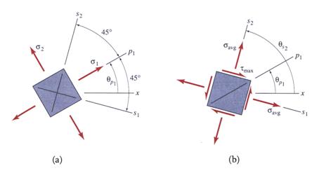
Figure 11 Relationships between Principal Planes and Maximum Shear Stress Planes
Note: From Figure 12.b it can be concluded that, in contrast, to the principal planes which are free of shear stress, the planes on which the shear stress achieves extreme values are not necessarily free of normal stresses.
Mohrs Circle for Plane Stresses
Mohrs circle is a graphical construction reflecting the variation of the plane state of stress around a particular point, including information pertinent to the principal and maximum shear stresses.
From equations (16) and (17), first squared and then summed, the following relation is obtained:
![]() (68)
(68)
Equation (68) represents the equation of a circle of radius![]() defined in the
defined in the ![]() plane. The center of
the circle is located at point
plane. The center of
the circle is located at point![]() . The values of circle radius
. The values of circle radius![]() and average normal stress
and average normal stress![]() are calculated employing equations (30) and (39), respectively.
are calculated employing equations (30) and (39), respectively.
Intersecting the equation of the circle (68) with the
horizontal axis ![]() the intersection points
the intersection points
![]() and
and ![]() are obtained:
are obtained:
![]() (69)
(69)
![]() (70)
(70)
It can be concluded that these intersection points represent
the principal stresses ![]() and
and![]() .
.
The Mohrs circle for plane stress condition is drawn
relative to a Cartesian system with the abscissa and the ordinate axis
representing the normal stresses ![]() and the shear stress
and the shear stress![]() , respectively. The following sign convention is employed as
illustrated in Figure 12:
, respectively. The following sign convention is employed as
illustrated in Figure 12:
(a) the positive shear stress![]() axis is downward;
axis is downward;
(b) the positive angle is measured counterclockwise;
(c) the shear stress on a face plots as positive shear if tends to rotate the face counterclockwise.
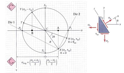
Figure 12 Mohrs Circle Notation
Note: The positive direction of the vertical axis, representing the
shear stress![]() , pointing downward (sign convention (a)) is elected in order
to be able to enforce the positive measurement of the angle (sign convention
(b)). Examining the notations shown in Figure 12 clarifies that all the angles
are measured from the line
, pointing downward (sign convention (a)) is elected in order
to be able to enforce the positive measurement of the angle (sign convention
(b)). Examining the notations shown in Figure 12 clarifies that all the angles
are measured from the line ![]() (
(![]() ) in the anticlockwise direction.
) in the anticlockwise direction.
Morhs circle for plane stress is constructed in the following steps:
(a) The coordinate system is drawn as shown in Figure 12. The horizontal
axis represents the normal stress ![]() , while the vertical axis represents the shear stress
, while the vertical axis represents the shear stress ![]() . To gain full advantage of the graphical benefits of the
method it is necessary that the drawing to be made on scale. However, the
method is also helpful as a conceptual tool in combination with the governing
equations wherein it may be drawn more roughly. The representation considers
that the following conditions are met:
. To gain full advantage of the graphical benefits of the
method it is necessary that the drawing to be made on scale. However, the
method is also helpful as a conceptual tool in combination with the governing
equations wherein it may be drawn more roughly. The representation considers
that the following conditions are met:![]() and
and ![]() ;
;
(b) Using the calculated values of the normal stresses![]() and
and![]() and the shear stress
and the shear stress![]() two points noted as
two points noted as![]() and
and![]() are placed on the drawing. The line
are placed on the drawing. The line ![]() intersects the
horizontal axis at point
intersects the
horizontal axis at point ![]() which represents the
center of the Mohrs circle;
which represents the
center of the Mohrs circle;
(c) The distance ![]() represents the radius of the circle. Using the radius
represents the radius of the circle. Using the radius ![]() and the position of the center
and the position of the center![]() the Mohrs circle is constructed. The intersection points,
the Mohrs circle is constructed. The intersection points, ![]() and
and![]() , between the circle and the horizontal axis
represent the maximum and the minimum principal stresses;
, between the circle and the horizontal axis
represent the maximum and the minimum principal stresses;
(d) The value of the ![]() can be calculated from
the graph. The angle
can be calculated from
the graph. The angle ![]() is identified on the
graph by the
is identified on the
graph by the ![]() angle and is measured
from the
angle and is measured
from the ![]() to the principal directions line in the counterclockwise
direction;
to the principal directions line in the counterclockwise
direction;
(e) The lines![]() and
and![]() represent the principal direction1 (associated with the
maximum principal stress) and 2 (associated with the minimum principal stress),
respectively.
represent the principal direction1 (associated with the
maximum principal stress) and 2 (associated with the minimum principal stress),
respectively.
Every point on the Mohrs circle corresponds to a pair of
stresses ![]() and
and ![]() on a particular face. To
emphasize the face involved the point is labeled identically with the face
where it belongs. For example, the face
on a particular face. To
emphasize the face involved the point is labeled identically with the face
where it belongs. For example, the face![]() ,
, ![]() and
and ![]() are represented on the Mohrs circle by the points
are represented on the Mohrs circle by the points![]() ,
, ![]() and
and![]() . To reinforce the shear stress sign convention (c) two icons
indicating the rotation sense induced by the shear stress are shown in Figure 12.
The angle measured from
. To reinforce the shear stress sign convention (c) two icons
indicating the rotation sense induced by the shear stress are shown in Figure 12.
The angle measured from ![]() to the radius line
to the radius line ![]() in the counterclockwise direction is equal to twice the angle
of the plane rotation
in the counterclockwise direction is equal to twice the angle
of the plane rotation ![]() .
.
Note: The points ![]() and
and![]() represent the case of orthogonal planes having normals
parallel to axes
represent the case of orthogonal planes having normals
parallel to axes ![]() and
and![]() , respectively. The line
, respectively. The line ![]() corresponds to angle
corresponds to angle ![]() . The double angle
. The double angle ![]() of the maximum
principal direction is measured from the line
of the maximum
principal direction is measured from the line ![]() to the line
to the line![]() . By these conventions, the double angle sense is established
as being positive in the counterclockwise direction. The angle
. By these conventions, the double angle sense is established
as being positive in the counterclockwise direction. The angle ![]() is the angle
is the angle ![]() and has the same
direction as the double angle
and has the same
direction as the double angle ![]() . The angle associated with the minimum direction
. The angle associated with the minimum direction ![]() is perpendicular to
the angle
is perpendicular to
the angle![]() . The stresses corresponding to a plane rotated with an angle
. The stresses corresponding to a plane rotated with an angle
![]() are obtained by
placing on the circle the radius
are obtained by
placing on the circle the radius![]() located by measuring in the counterclockwise direction an
angle of
located by measuring in the counterclockwise direction an
angle of ![]() from the line
from the line![]() . The corresponding stresses
. The corresponding stresses ![]() and
and![]() are a function of the location of the point
are a function of the location of the point![]() position in the
position in the ![]() coordinate system and may be obtained by scaling them from
the figure or by the use of the analytical equations (30), (39) and (68). The
opposite point
coordinate system and may be obtained by scaling them from
the figure or by the use of the analytical equations (30), (39) and (68). The
opposite point ![]() represents the stresses on the orthogonal rotated face.
represents the stresses on the orthogonal rotated face.
In comparison with the
technique used to show the principal axes in the ![]() representation
(Figures 7 through 11) the plot obtained from the Mohrs circle appears to be
misleading. The cause is that the Mohrs circle is drawn in the
representation
(Figures 7 through 11) the plot obtained from the Mohrs circle appears to be
misleading. The cause is that the Mohrs circle is drawn in the ![]() coordinate system. In
the
coordinate system. In
the ![]() representation the principal directions are correctly plotted
by artificially rotating the principal directions obtained from the Mohrs
circle around the point
representation the principal directions are correctly plotted
by artificially rotating the principal directions obtained from the Mohrs
circle around the point ![]() with an angle
with an angle ![]() measured in the
counterclockwise direction.
measured in the
counterclockwise direction.
Principal Stresses Distribution in Beams
One of the most important applications of the plane state of
stress theory described above is found in the study of variation of the
stresses in beams under non-uniform bending. Recall from Lecture 7 that under
some imposed kinematic assumptions, a beam subjected to transversal loading is
in a state of plane stress. With the exception of some areas (around the
supports or the application points of concentrated loads) the beam theory characterizes
the existence of only two types of stresses: normal stress ![]() and shear stress
and shear stress![]() . The normal stress
. The normal stress![]() is calculated using Naviers formula expressed by equation (71),
while the shear stress
is calculated using Naviers formula expressed by equation (71),
while the shear stress ![]() is obtained employing Jurawskis formula contained in
equation (72):
is obtained employing Jurawskis formula contained in
equation (72):
![]() (71)
(71)
 (72)
(72)
The notation used in the formulae (71) and (72) is explained in Lecture 7 and is not repeated herein.
The plane stress tensor previously expressed in equation (9) is written for the case of the beam in nonuniform bending as:
 (73)
(73)
The entire theoretical development described in the previous sections can be without restriction applied to the study of the particular plane stress tensor (73). Consequently, the variation of the stresses around any point in a beam subjected to nonuniform bending can be calculated. Figure 13 represents an example of the application of plane stress theory for the case of a simply supported beam.
In the example, the beam has a rectangular cross-section and
is subjected to a single concentrated force ![]() located at the
mid-span. It is evident that the ratios of the beam dimensions and the loading
do not violate any of the assumptions related to the applications of the formulae
(71) and (72). The shear force diagram
located at the
mid-span. It is evident that the ratios of the beam dimensions and the loading
do not violate any of the assumptions related to the applications of the formulae
(71) and (72). The shear force diagram ![]() and the bending diagram
and the bending diagram![]() , where the axis identification indices were dropped for
clarity, are plotted.
, where the axis identification indices were dropped for
clarity, are plotted.
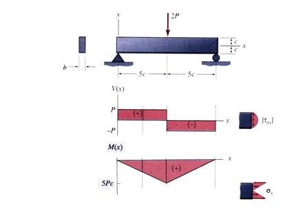
Figure 13 Simple Supported Beam
The geometrical characteristics of the rectangular cross-section involved in the evaluation of the formulae (71) and (72) are:
![]() (74)
(74)
![]() (75)
(75)
![]() (76)
(76)
For the left half of the beam ![]() the shear force
the shear force ![]() and the bending moment
and the bending moment ![]() are expressed as:
are expressed as:
![]() (77)
(77)
![]() (78)
(78)
Substituting equations (74) through (78) into equations (71) and (72), the expressions for normal and shear stresses are obtained as:
 (79)
(79)
 (80)
(80)
Note: The minus (-) sign appearing in formula (81) has been inserted in order to comply with the shear sign convention (c).
To obtain an illustrative variation of the principal
stresses, the rectangular domain of the beam is divided by superimposing a
rectangular mesh. For the case under study, the mesh has five spaces in the longitudinal
![]() direction and eight
spaces in the vertical
direction and eight
spaces in the vertical ![]() direction. Using
Mathcad programming capabilities the principal stresses and corresponding
angular directions can be easily calculated for every point of the mesh. The
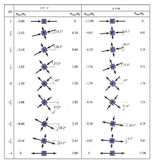
principal stresses calculated for two cross-sections
direction. Using
Mathcad programming capabilities the principal stresses and corresponding
angular directions can be easily calculated for every point of the mesh. The
principal stresses calculated for two cross-sections![]() and
and ![]() and all nine points
vertically describing the cross-sections are contained in Table 1. The ratios
and all nine points
vertically describing the cross-sections are contained in Table 1. The ratios ![]() and
and ![]() are tabulated instead of the
are tabulated instead of the ![]() and
and![]() , where
, where![]() .
.
A review of the results presented in Table 1 shows that at
the extreme fibers the principal stresses correspond with the normal stresses
and reach the maximum values. At the extreme fiber locations the shear stress ![]() is zero. The situation is different for the case of
wide-flange beams where both
is zero. The situation is different for the case of
wide-flange beams where both ![]() and
and ![]() have significant values at the junction between the web and
the flange.
have significant values at the junction between the web and
the flange.
Table 1
Today, with the help of modern computer codes, the formulae involved in the calculation of the principal stresses and directions can be computed using a very refined mesh. The graph containing the curves tangent to the principal directions in every point of the mesh is called the stress trajectory. Two sets of curves are drawn and they are orthogonal at every point. The stress trajectory graph pertinent to the simply supported beam investigated above is pictured in Figure 14. A typical example of practical usage of the stress trajectory curves is the placement of the reinforcement in reinforced concrete beam. Because the stress trajectory graph does not give any indication about the magnitude of the principal stresses another type of graph is also used. This is called a stress contour plot and contains curves of equal principal stress magnitudes. The commercial codes employed today can provide these plots.
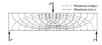
Figure 14 Stress Trajectory Plot
Example
The theoretical formulation derived above is used to investigate the following practical case:
![]()
![]()
![]()
![]()
![]()
![]()
The corresponding stress tensor is written as:
![]()
The state of stress for the case above is shown in Figure 13.
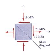
Figure 13
The following values illustrated in Figure 13 are calculated as:
![]()
![]()
![]()
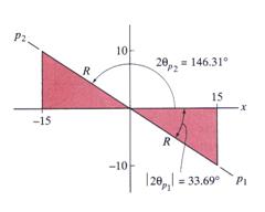
Figure 14 Geometrical Relations
From equation (47) it is established that the angle related to the maximum principal direction must have a negative tangent. Consequently, the angles of the principal direction are:
![]()
![]()
The principal stresses, shown in Figure 15, are obtained as:
![]()
![]()
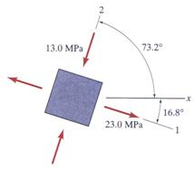
Figure 15 Principal Stresses
The angle of the maximum shear stresses is calculated as:
![]()
The maximum shear stresses are calculated as:
The normal stresses acting on the maximum shear planes are calculated as:
![]()
![]()
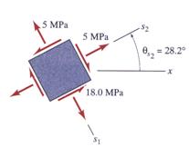
Figure 16 Maximum Shear Stresses
The maximum shear stresses and the corresponding normal stresses are illustrated Figure 16
Morhs circle pertinent to the problem is illustrated in Figure 17.
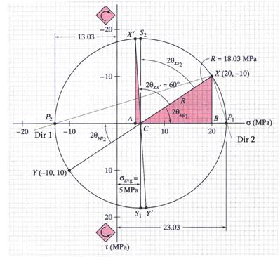
Figure 17 Mohrs Circle
Note: The points ![]() and
and ![]() represent the case of
orthogonal planes having the normal directions rotated with angles of
represent the case of
orthogonal planes having the normal directions rotated with angles of ![]() and
and ![]() , respectively, from the
, respectively, from the ![]() axis. Successively substituting
the above angular values in equations (16) and (18) the following stresses pertinent
to points
axis. Successively substituting
the above angular values in equations (16) and (18) the following stresses pertinent
to points ![]() and
and ![]() are obtained:
are obtained:
for ![]()
![]()
![]()
for ![]()
![]()
![]()
|
Politica de confidentialitate | Termeni si conditii de utilizare |

Vizualizari: 3950
Importanta: ![]()
Termeni si conditii de utilizare | Contact
© SCRIGROUP 2025 . All rights reserved