| CATEGORII DOCUMENTE |
| Bulgara | Ceha slovaca | Croata | Engleza | Estona | Finlandeza | Franceza |
| Germana | Italiana | Letona | Lituaniana | Maghiara | Olandeza | Poloneza |
| Sarba | Slovena | Spaniola | Suedeza | Turca | Ucraineana |
Testing CAPM on stocks traded at
One of the most important debates in capital markets nowadays is whether the Capital Asset Pricing Model is still valid of not. Sharpe (in 1965) and Lintner (1966) constructed the well-known model CAPM that shows that the true measure of risk for stocks is the beta. In the following period, many studies have supported this approach, but also some other criticized the model (see Fama and French). The question that is being frequently asked today is: Is Beta dead? Fama and French have argued that beta cannot be considered anymore a true measure of risk and that some empirical evidence has proved that the slope of equation used in CAPM is negative.
Also, some authors in the capital markets literature (see R. H. Campbell) have argued that in the case of emerging stock exchanges the CAPM is inapplicable and beta is not significant.
The present study analyzes the value of CAPM in the case of Bucharest Stock Exchange. It is supposed to check whether investors can trust beta in their decision-making process or not.
Key words: CAPM, beta, returns of stocks, risk, estimation of residuals
Literature review
The modern portfolio theory was first developed by Markowitz, who constructed the mean-variance model. The model was designed to construct the optimal portfolio based on idea that between risk and return there is a positive relation. For his work, Markowitz received Nobel Prize in 1990. He proved that investors should create their portfolio in order to offer them a maximum level of return for a given level of risk or, a minimum level of risk for a given level of return.
Markowitz shown in his theory that stocks are related to each other and that the risk can be decreased through diversification. The proof is very simple: if one takes 2 stocks and he will calculate the correlation coefficient, the value of this coefficient would be less than one and if the respective stocks are included in a portfolio, the overall risk of this portfolio would decrease.
Even though the theory of Markowitz was spectacular and useful in this field, it had some inconveniences. For instance, it is done taking into account a very abstract concept in Economics, i.e. utility. The economical practice has shown that the models constructed based on the idea of utility are very difficult or even impossible to be applied. Also, the mathematics beyond of the Mean-Variance is very sophisticated, which makes the application to be very difficult when portfolio consist of a great number of shares. Specifically, to estimate the benefits of diversification would require that practitioners calculate the covariance of returns between every pair of assets, which is very difficult. Finally, the critics of the model said that its a static one, which makes the results to be biased.
In 1964 (Sharpe) and in 1965 (Lintner) continued the work of Markowitz and constructed the famous Capital Asset Pricing Model (CAPM). Basically, the model was developed to explain the differences in risk premium across assets. The CAPM shows clearly that these differences are generated by the differences in the riskiness of assets, i.e. the higher the risk of an asset the higher the risk premium demanded by investors.
The general equation of the model is:
![]()
where:
![]() - expected return of stock i
- expected return of stock i
relative risk of share i
![]() - expected return of the market portfolio
- expected return of the market portfolio
rf risk-free interest rate
What CAPM says is that the equilibrium in the capital markets is characterized by only 2 numbers:
The return for waiting, i.e. rf ;
The extra
return, i.e. ![]() - rf..
- rf..
A very important consequence of this model is the separation theorem, which says that in the capital markets the risk has two components: diversifiable (or non-systematical) risk and non-diversifiable (systematical) risk. When pricing, the only significant risk is the systematic one, since investors can just get rid of the non-systematic risk through diversification. Sharpe&Lintner show that the true measure of risk is the well-known coefficient beta
Empirical evidence was in favor of CAPM and the model became extremely famous in the modern portfolio theory. Things were clear: stocks with beta lower than 1 were considered passive stocks and stocks with beta higher than 1 were considered aggressive and risky. Depending on their appetite toward risk, investors would choose the stocks in their portfolio according to the value of beta.
Though, some criticisms of CAPM appeared. One very known critic in literature belongs to Fama and French. In 1992, they discovered a negative relationship between risk and return. Since then, a very important question is being asked: Is Beta dead? . And if the answer is yes, what is the true nature and measure of risk? Fama and French came up with the conclusion that a more realistic approach of the risk in the market is the multi-index models. They argued that size of the firm and the book to market value have a significant influence on the performance of a stock.
Is Beta dead?
Sharpe defended his model by saying that beta is not dead at all. In fact, even the multi-index model realized by Fama&French in1993 does not eliminate beta, but it just adds some other variables. Sharpe suggested that to think that stocks returns are not related to market portfolios returns is a mistake and misleading. He agrees that CAPM does not reflect the whole reality of the market, but it is very important as a guide for investors. In an interview appeared in Dow Jones Asset Manager (May/June, 1998) Sharpe answered at this question by saying that The CAPM is not dead. Anyone who believes markets are so screwy that expected returns are not related to the risk of having a bad time, which is what beta represents, must have a very harsh view of reality. He continues: 'Is beta dead?' is really focused on whether or not individual stocks have higher expected returns if they have higher betas relative to the market. It would be irresponsible to assume that is not true. That doesn't mean we can confirm the data. We don't see expected returns; we see realized returns. We don't see ex-ante measures of beta; we see realized beta. What makes investments interesting and exciting is that you have lots of noise in the data. So it's hard to definitively answer these questions. Sharpe believes that CAPM is not dead, but it needs revising.
In favour of CAPM other opinions came. These opinions are against of the study realized by Fama and French in 1992. It is said that beta has no role to explain the cross-sectional variation in returns. Also, the results of their study were criticized (see Kothari, Shanken and Sloan - 1995).
The conclusion of all these issues is that while the academic debate continues, the CAPM may still be useful for those interested in the long run.
Data and methodology
The present case is realized by using data about companies traded in the Bucharest Stock Exchange (BSE). Source of data is Bucharest Stock Exchange. It was used the interval between 1.01.1999 and 5.11.2001. There was used daily data.
As the market portfolio it was used a proxy: BET index for companies traded in the first tier and BET-C for the companies included in the second tier. The sample includes almost all companies traded in the market in the year 2002. There were excluded the investment funds and 2 companies: SNP Petrom and Abrom Barlad, for which the data was not sufficient.
A proxy of CAPM was used, i.e. the single-index model, since the purpose of the study was to test the power of beta as measure of risk and not to evidentiate the risk premium.
First step was to compute returns. The study uses daily returns. It is assumed that prices follow a log-Normal distribution. It is not used the assumption of Normal distribution of the prices, since the Normal distribution does not exclude negative values. Also, recent studies have shown that stocks prices follow rather a log-Normal distribution and returns a Normal distribution. This is the reason that the formula in calculating daily returns is:
ri = logPt logPt-1
where:
ri the return of stock i
Pt price of a stock in the day t
Pt-1 price of a stock in the day t-1
As price, it has been used the closing price.
The following step was to regress individual stocks returns on market index return. The results are analysed mainly by taking into account the following econometrical measures:
The coefficient t-statistic to measure the level of the significance of beta (it is used since the assumed distribution of stocks returns is normal);
Adjusted R-squared used to check the goodness of the model (it is used adjusted R-squared rather than R-squared the number of observations exceeds in some cases even 600);
Durbin-Watson coefficient to check for serial in residuals;
Pattern of residuals to check the noise in data.
Results and analysis
First Tier
Let us first take a look at t-statistic and adjusted R-squared. We want to see how much is beta relevant as a measure for relative riskiness. Let us analyse the companies traded in the first tier. The results are presented in the following table:
Table : Beta and Adjusted R-square for stocks traded at Tier I
|
SYMBOL |
Alpha Coefficient (t-statistic) |
Beta Coefficient (t-statistic) |
Adjusted R-squared |
|
ALR |
(-0.24) (p=0.80)* |
(6.66) (p=5.91114E-11) |
0.065 |
|
ARC |
(-1.03) (p=0.30) |
(4.87) (p=0.000) |
0.033 |
|
ATB |
0.0002 (0.45) (p=0.65) |
(2.75) (p=0.006) |
0.009 |
|
ASP |
6.5E-05 (0.06) (p=0.95) |
(1.60) (p=0.11) |
0.003 |
|
AZO |
(1.13) (p=0.26) |
(3.93) (p=9.56013E-05) |
0.023 |
|
BRD |
(-0.76) (p=0.45) |
(3.13) (p=0.002) |
0.045 |
|
TLV |
2.57E-05 (0.04) (p=0.96) |
(3.79) (p=0.001) |
0.019 |
|
OLT |
(0.23) (p=0.82) |
(-3.30) (p=0.001) |
0.015 |
|
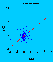
INX |
(1.87) (p=0.06) |
(1.33) (p=0.188) |
0.002 |
|
RLS |
(-0.20) (p=0.83) |
(0.004) (p=0.996) |
-0.003 |
|
RBR |
(0.53) (p=0.60) |
(0.53) (p=0.599) |
0.002 |
|
TER |
(-0.39) (p=0.69) |
(8.61) (p=0.000) |
0.106 |
|
TBM |
-0.0024 (-1.00) (p=0.31) |
(2.78) (p=0.006) |
0.048 |
*probability related to t-statistic, i.e. the level of significance
What we see from these results is that for most of the companies traded in the first tier the betas are significant at a level of 10% or even 5%. This means that the market has a relevant influence on stocks performance. According to this information, beta is a good measure of risk. And if we read the values, we would say that the stocks are not very risky. There is not even one stock that has a beta higher than one. So, Bucharest Stock Exchange could be a good environment for investors with a low appetite toward risk. Their investment for an horizon of about 3 years would be quite safe.
But the next question that arises is: How good is beta? I.e. in which proportion does it cover the whole risk? For answering this, we need to be careful about the goodness of the model. So, lets take a closer look at adjusted R-squared. When we look at the values of this coefficient, we start doubting about the power of beta. More specifically, except the company Terapia Cluj Napoca, for all other stocks the adjusted R-squared is below 0.10. And taking into account that we work with continuous data this is a very low value. So beta explain the model only in a proportion less than 10%. More than this, even the constant terms (in our table noted with Alpha coefficient) are not relevant at all. The values of t-statistic are extremely low. So this led as at the conclusion that there is too much noise in data. We mean that there are other factors that have a great influence on stocks s returns.
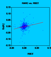
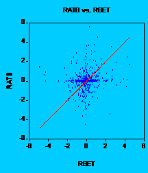
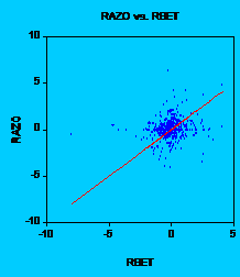
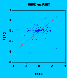
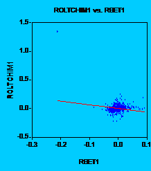
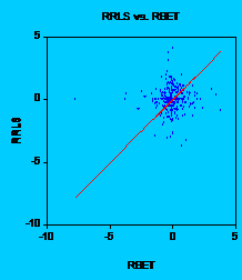
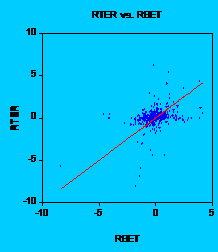
In
order to see this, let us take an example. Let us examine the stock Alro
Slatina. If we take a look at the graph, we can understand why t-statistic is
high, but adjusted R-square is so low. Without no doubt, OLS (
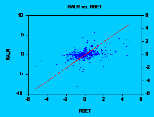
Fig. 1: Alros return regressed on BETs return
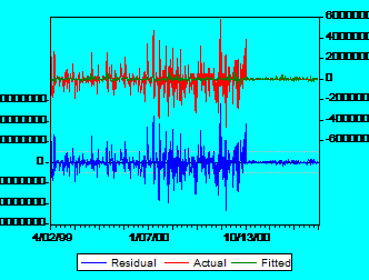
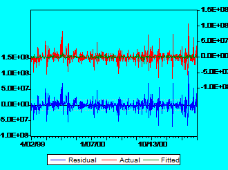
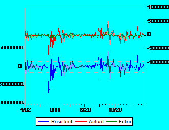
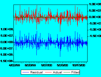
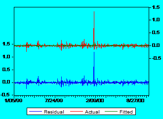
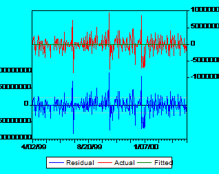
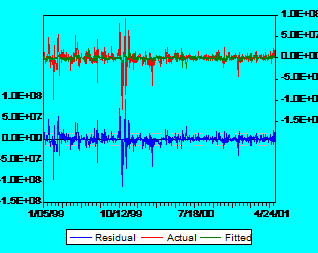
It is obvious that there is too much noise in data. In order to see that major influence of the residuals let us consider another graph:
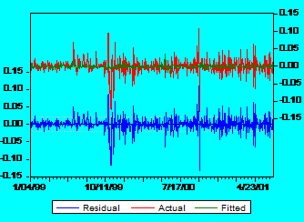
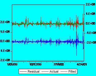 Fig
2: Actual, Fitted, Residual graph for Alro
Fig
2: Actual, Fitted, Residual graph for Alro
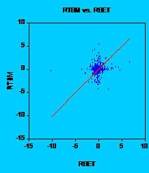
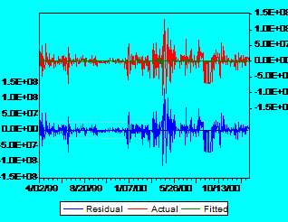
It is very clear that the pattern of the residuals is the same with the pattern of observed returns for Alros stock. The green line doesnt fit very well the red line, which is a very good proof that beta has a low explanatory power. Similar results have been noted for all stocks from both tiers (all graphs are presented in the appendix 1).
So, is beta dead in our case? The answer doesnt seem to be so easy. If we take into account only beta, we would rather fail when investing in stocks. And why is that? Values are low, which leads us to say that the risk is low, so we are safe in investing. But if we look at adjusted R-square and graphs, we see that residuals are very important and there is a high volatility, so we had better be careful when choosing stocks. The daily data shows that there are periods when we can increase/decrease our wealth rapidly. So, we should not be very happy with the low value of beta in the case that we dont like very much the risk.
A more detailed analysis on residuals has been done taking into account ANOVA (Analysis of Variance) method and statistic Durbin-Watson coefficient (in order to check for the presence of serial correlation in the residuals). The values are presented in the following table:
Table : ANOVA ANALYSIS and D-W coefficient for stocks traded in Tier I
|
Symbol |
S.E. of Regression |
Residual Sum of Squares |
F-statistic |
Durbin-Watson |
|
ALR |
(p=5.91114E-11)* | |||
|
ARC |
0.010339 |
0.282094 |
(p=0.00001) | |
|
ATB |
(P=0.0017) | |||
|
ASP |
(P=0.1091) | |||
|
AZO |
(p=0.00007) | |||
|
BRD |
(p=0.0001) | |||
|
TLV |
(p=0.0044) | |||
|
OLT |
(p=0.0010) | |||
|
INX |
2.52 (p=0.1129) | |||
|
RLS |
1.16E-08 |
(p=0.8941) | ||
|
RBR |
(p=0.1739) | |||
|
TER |
0.022595 |
0.19022 |
(p=0.0000) | |
|
TBM |
2.80 (p=0.0947) |
*probability attached to F-statistic
The data from the table indicates that the residuals cover basically almost all the influence on stocks s returns. And this is proved statistically for the great part of the companies.
The analysis of the residuals includes also the Durbin-Watson statistic test. Durbin-Watson (DW) statistic is as a part of the standard regression output. The Durbin-Watson statistic is a test for first-order serial correlation. More formally, the DW statistic measures the linear association between adjacent residuals from a regression model. The Durbin-Watson is a test of the hypothesis ρ=0 in the specification:
![]()
If there is no serial correlation, the DW statistic will be around 2. The DW statistic will fall below 2 if there is positive serial correlation (in the worst case, it will be near zero). If there is negative correlation, the statistic will lie somewhere between 2 and 4. Usually the limit for non-serial correlation is considered to be DW=(1.8;2.2). A very strong positive serial correlation is considered at DW lower than 1.5. For our sample there is strong positive correlation among the variables only for stocks of Romanian Bank of Development, Transilvania Bank and Terapia.
Second Tier
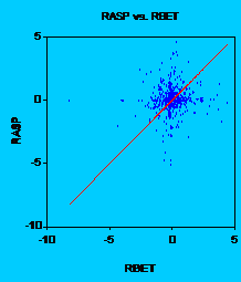
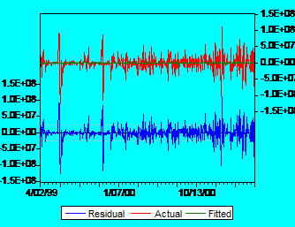
The results for companies traded in the second tier are given in the appendix 2 for t-statistic and adjusted R-squared and in the appendix 3 for analysis of the residuals respectively.
We could say that results obtained for the companies traded at the second tier are similar to those obtained for companies that belong to the first tier. The main difference is that for more companies the beta is not significant. So, for the second tier, beta loses more of his power when measuring risk. Another finding is that adjusted R-squared has a very small value for all companies, so that even when beta is statistically significant, it explains the model in proportion of less than 10%. The low power of beta is proved also when testing the residuals. We definitely notice that there is an extremely large quantity of noise in data.
Finally, the Durbin-Watson coefficient indicates that in general there is no evidence of powerful serial correlation of the residuals.
4. Further work to be done
One question arises from this study: if beta does not reflect the risk in the market very well and then what is the most powerful measure of risk and how investors could guide in their decisions? The immediate answer could come from Fama and French, i.e. one could use multi-index models. We could take into analysis the size effect of the firm and the book to market value. Also, we could add some elements that are related to firms themselves (debts, turnover and so on).
Also, we might obtain different results if we take another interval of time into consideration. Many studies have proved that depending on how we choose data, we could get other results. So, we can analyse the power of beta by taking an interval of 5 years and by computing monthly returns.
Final remarks
What we can conclude from this study? Is CAPM valid for Bucharest Stock Exchange? We should emphasize first that CAPM has been debating that risk is correlated to return, i.e. there is a positive relation between them. If we look at the sign of beta, we notice that risk is related to return and CAPM has passed a first step. However, the power of beta as estimate of risk is not very high (see adjusted R-squared).
A question that comes here is: why is that? Well, we can debate several things here. First, we should tell that being an emerging market there are many zeros in data (especially at the second tier when the number of observations falls in some cases to 150-180). This can affect the pattern of returns. Also, it has been shown that emerging markets tend to offer contradictory results because of lack of integration (see R. H. Campbell).
Finally, we could conclude by saying that we need to be careful about beta when making investments. I.e. at the first look, stocks are not so risky (when we analyse beta), but the ANOVA analysis indicates rather a relative high risk of them.
Appendix 1 : Stocks returns regressed on BETs return and the pattern of residuals for stocks traded at tier I
Appendix 2: The alpha and beta coefficients for stocks traded at tier II
|
SYMBOL |
Alpha Coefficient (t-statistic) |
Beta Coefficient (t-statistic) |
Adjusted R-square |
|
AMO |
0.001 (0.94) (p=0.3462)* |
(1.01) (p=0.3124)** |
0.00004 |
|
AMP |
(1.35) (p=0.1776) |
0.22 (0.9056) (p=0.3660) |
0.006 |
|
APC |
6.22E-05 (0.06) (p=0.9455) |
0.17 (1.57) (p=0.1168) |
0.003 |
|
ARM |
0.004 (1.33) (p=0.1828) |
(-0.21) (p=0.8369) |
9.01E-05 |
|
ARS |
(1.25) (p=0.2120) |
-0.18 (-1.38) (p=0.1699) |
0.002 |
|
ART |
(0.52) (p=0.6054) |
(1.52) (p=0.1300) |
0.004 |
|
ASA |
-0.0008 (-0.24) (p=0.8132) |
0.71 (2.85) (p=0.0051) |
0.059 |
|
BRM |
(1.48) (p=0.1393) |
(2.44) (p=0.0149) |
0.007 |
|
CBC |
0.0005 (0.34) (p=0.7318) |
(1.74) (p=0.0825) |
0.007 |
|
CMF |
(1.39) (p=0.1674) |
0.43 (2.15) (p=0.0337) |
0.027 |
|
CMP |
0.59 (0.82) (p=0.4115) |
(2.98) (p=0.0030) |
0.012 |
|
|
(0.86) (p=0.3896) |
(0.52) (p=0.6062) |
-0.006 |
|
CPL |
-0.0002 (-0.10) (p=0.9163) |
0.70 (2.79) (p=0.0057) |
0.029 |
|
CPR |
-6.65E-06 (-0.006) (p=0.9955) |
0.36 (2.81) (p=0.0051) |
0.016 |
|
CRB |
0.001 (0.08) (p=0.9378) |
(3.22) (p=0.0014) |
0.023 |
|
DOR |
0.001 (0.70) (p=0.4831) |
(2.22) (p=0.0282) |
0.024 |
|
ECT |
0.0011 (0.05) (p=0.9591) |
-4.09 (-3.71) (p=0.0004) |
0.159 |
|
ELJ |
0.0001 (0.20) (p=0.84) |
(3.24) (p=0.0012) |
0.014 |
|
ENP |
(1.13) (p=0.2580) |
-0.10 (-0.57) (0.5723) |
-0.003 |
|
EPT |
(1.46) (p=0.1459) |
(0.61) (p=0.5421) |
-0.001 |
|
EXC |
0.0009 (0.33) (p=0.7393) |
(0.56) (p=0.5767) |
-0.006 |
|
HTR |
-0.057 (-0.51) (p=0.6107) |
-0.04 (-0.26) (p=0.7892) |
-0.002 |
|
IMP |
-0.0001 (-0.85) (p=0.3975) |
(2.73) (p=0.0066) |
0.012 |
|
IMS |
(0.61) (p=0.5391) |
0.16 (1.06) (p=0.2891) |
0.0003 |
|
MEF |
0.003 (2.05) (p=0.0412) |
(1.20) (0.2327) |
0.001 |
|
MJM |
-0.002 (-0.97) (p=0.3359) |
0.28 (0.88) (p=0.3784) |
-0.002 |
|
MPN |
-0.0006 (-0.44) (p=0.6589) |
(0.87) (p=0.3846) |
-0.0007 |
|
NVR |
(1.58) (p=0.1136) |
(1.86) (p=0.0630) |
0.004 |
|
OIL |
-0.003 (-0.50) (p=0.6182) |
(7.11) (p=0.0000) |
0.085 |
|
PCL |
-0.0003 (-0.40) (p=0.6875) |
(3.29) (p=0.0011) |
0.015 |
|
|
0.0002 (0.30) (p=0.7678) |
(3.12) (p=0.0019) |
0.015 |
|
PPL |
(0.87) (p=0.3818) |
(1.86) (p=0.0638) |
0.005 |
|
PTR |
-0.003 (-0.79) (p=0.4324) |
-1.03 (-2.25) (p=0.025) |
0.011 |
|
PTS |
(0.76) (p=0.4467) |
(4.76) (p=0.0000) |
0.045 |
|
SCD |
0.0004 (0.81) (p=0.4166) |
(2.31) (p=0.0213) |
0.006 |
|
SLC |
0.0008 (0.50) (p=0.6143) |
(1.80) (p=0.0731) |
0.007 |
|
SNO |
-0.015 (-0.09) (p=0.9303) |
(5.30) (p=0.0000) |
0.090 |
|
SOF |
0.0005 (0.33) (p=0.7390) |
(2.15) (p=0.0318) |
0.008 |
|
SRT |
(0.11) (p=0.9094) |
(3.18) (p=0.0016) |
0.026 |
|
STZ |
0.0002 (0.26) (p=0.7913) |
(0.92) (p=0.3576) |
-0.0002 |
|
TRS |
-0.005 (-0.82) (p=0.4129) |
(2.86) (p=0.0044) |
0.013 |
|
UAM |
7.03E-05 (0.06) (p=0.9535) |
(1.38) (p=0.1674) |
0.002 |
|
UCM |
0.002 (1.59) (p=0.5531) |
(0.04) (p=0.9693) |
-0.007 |
|
VEL |
-0.011 (-1.13) (p=0.2539) |
(1.28) (p=0.2026) |
0.001 |
|
ZIM |
(1.41) (p=0.1611) |
0.19 (1.64) (p=0.1027) |
0.008 |
*level of significance for alpha coefficient
**level of significance for beta coefficient
Appendix3: ANOVA analysis and Durbin-Watson coefficient for stocks traded at tier II
|
Symbol |
S.E. of Regression |
Residual Sum of Squares |
F-statistic |
Durbin-Watson Coefficient |
|
AMO | ||||
|
AMP | ||||
|
APC | ||||
|
ARM |
3.25E-05 | |||
|
ARS | ||||
|
ART | ||||
|
ASA | ||||
|
BRM | ||||
|
CBC | ||||
|
CMF | ||||
|
CMP | ||||
|
| ||||
|
CPL | ||||
|
CPR | ||||
|
CRB | ||||
|
DOR |
|
|
|
|
|
ECT | ||||
|
ELJ | ||||
|
ENP | ||||
|
EPT | ||||
|
EXC |
|
| ||
|
HTR |
1.37E-06 | |||
|
IMP | ||||
|
IMS | ||||
|
MEF | ||||
|
MJM | ||||
|
MPN | ||||
|
NVR | ||||
|
OIL | ||||
|
PCL | ||||
|
| ||||
|
PPL | ||||
|
PTR | ||||
|
PTS | ||||
|
SCD | ||||
|
SLC | ||||
|
SNO | ||||
|
SOF | ||||
|
SRT | ||||
|
STZ | ||||
|
TRS | ||||
|
UAM | ||||
|
UCM |
2.3E-06 | |||
|
VEL | ||||
|
ZIM |
References:
Edwin J. Elton, Martin J. Gruber, Modern Portfolio Theory and Investment Analysis, The Fifth Edition, John Wiley&Sons, 1995
James L. Farrel Jr., Portfolio Management, The second Edition, Irwin McGraw-Hill, 1997
Eugene F. Fama, James McBeth, Risk, return and equilibrium: empirical tests, Journal of Political Economy, vol. 81, no. 3, 1973
Eugene F. Fama, Efficient capital markets: A review of theory and empirical work, Journal of Finance, vol. 25, 1970
Harvey R. Campbell, Predictable risk and returns in emerging markets, Review of Financial Studies 8, 1995
Ravi Jagannathan, Ellen R. McGrattan, The CAPM debate, Federal reserve Bank of Minneapolis Quarterly Review, no. 19, 1995
John Lintner, The valuation of risk assets and the selection of risky investments in stock portfolios and capital budgets, Review of Economics and Statistics, vol. 47, 1965
William Sharpe, Capital asset prices: A theory of market equilibrium under conditions of risk, Journal of Finance, vol. 19, 1964
William Sharpe, Revisiting Capital Asset Pricing Model, Dow Jones Asset Management, May/June 1998
|
Politica de confidentialitate | Termeni si conditii de utilizare |

Vizualizari: 1499
Importanta: ![]()
Termeni si conditii de utilizare | Contact
© SCRIGROUP 2025 . All rights reserved