| CATEGORII DOCUMENTE |
| Bulgara | Ceha slovaca | Croata | Engleza | Estona | Finlandeza | Franceza |
| Germana | Italiana | Letona | Lituaniana | Maghiara | Olandeza | Poloneza |
| Sarba | Slovena | Spaniola | Suedeza | Turca | Ucraineana |
Engineering Mathematics - Random Signals Project
Introduction:
This project examines students’ skills in matlab applications in solving mathematical problems through the use of provided random data. In particular the Blackman-Tukey approach was practiced to estimate the power spectral density of the given random data.
Given Random Data:
Question 1:
A derivation for your theoretical power spectral density function. You should take the z-transform of the difference equation given in your data Żle to get X[z] = H[z]W[z], then the power spectral density comes from SXX[z] = H[z]H[1=z]SWW[z], where W is white noise, so SWW[z] = S0, the variance of the white noise. You should Żfinally substitute z = ej2Ľm=N to get SXX[m] as a DFT. Express the power spectral density in terms of trigonometric functions. Let Matlab do some of this work for you.
Please see attached
handwritten answer.
Question 2:
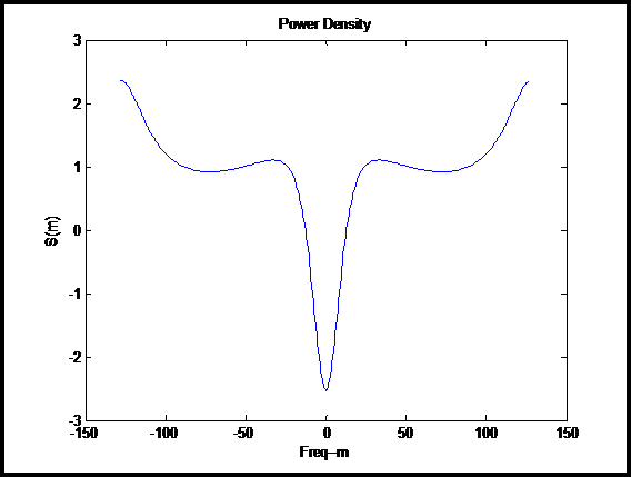
The graph of the theoretical power spectral density function. The plot should be done for ˇ128 · m · 127 (N = 256 for your data Żle), and if your graph is extremely spiked, you may want to consider using a logarithmic y axis using the Matlab function semilog instead of plot.
Question 2:
Figure 1
Question 3:
A graph of the time function itself. Matlab commands like fscanf, load, or reshape might be useful in reading in the data. Be aware that the data are to be read row-wise. The plot should have time values 1 to 256.
Question 3:
Figure 2
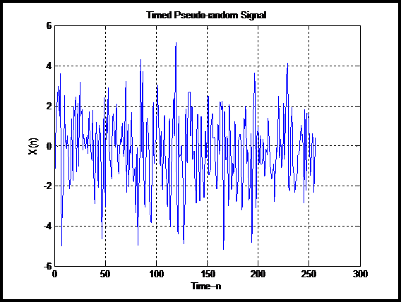
The above plot describes the appearance of white noise, better known and described as “coloured noise”.
Question 4:
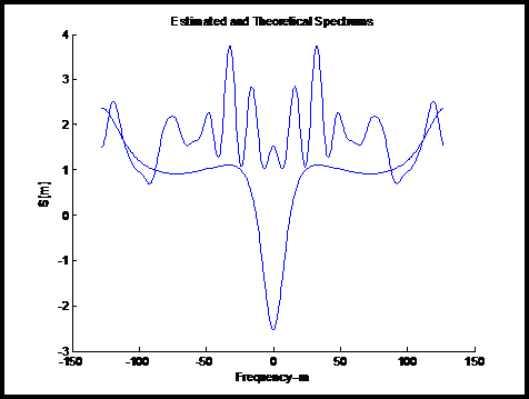
A graph of the sample power spectral density (spsd). This is the square of the absolute value of the Fast Fourier Transform (fft) of the time function, divided by N. Due to the nature of the Matlab fft function, the plot should map the values of the spsd from m = 1 to 128 onto 0 to 127, and those from 129 to 256 should be mapped to ˇ128 to ˇ1 | but do not actually change the position of values in the spsd. There is a Matlab function fftshift which may prove useful to produce the correct plot. You may want to include the theoretical power spectral density on the same graph for comparison purposes.
Question 4
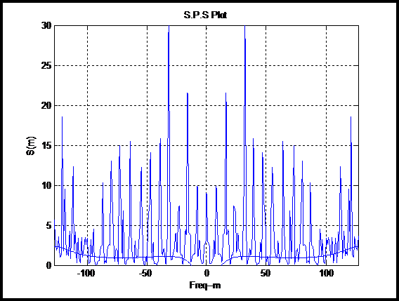 Figure 3
The signal spectrum is estimated by taking the square of the absolute value of the FFT of the given (plotted) time function and then be divided over the given value.
Question 5:
A graph of the sample auto covariance function. This is the inverse Fast Fourier Transform (ifft) of the spsd, and you should map points in the plot as for the spsd.
Question 5
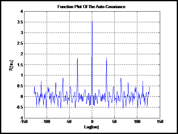 Figure 4
This graph is of the auto-covariance function produced as a result of inversing the initial FFT of the power spectral density function.
Question 6:
Graphs of a number of estimates of the power spectral density using different smoothing windows and different window widths. You are required to write the code for the windows yourself, rather than use the Matlab built-in functions. You will find that only by doubling or halving the window width do you see any sensible change in the smoothed spectrum, so you may wish to use widths which are a power of two. You should include three window functions at their best widths and three widths for the best window. Include extra graphs only if you have a good reason. Note that due to the positioning of data for use with the FFT routines, a window from ˇM to +M will actually have values from 1 to M and from N ˇM to N.
Question 6
Figure 5
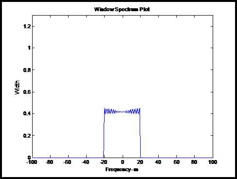
Figure 6
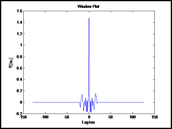
Figure 7

** Figure 5
Raisedcosine

Figure 6
Raisedcosine
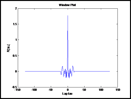
Figure 7
Raisedcosine
** Figure 5
hamming

Figure 6
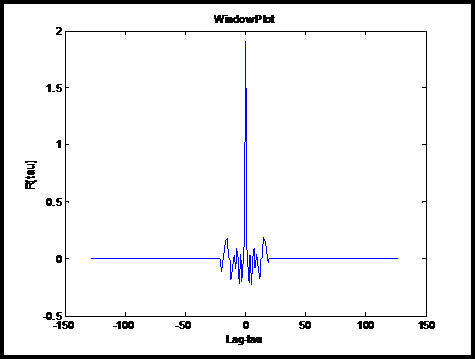 Hamming
Figure 7
Hamming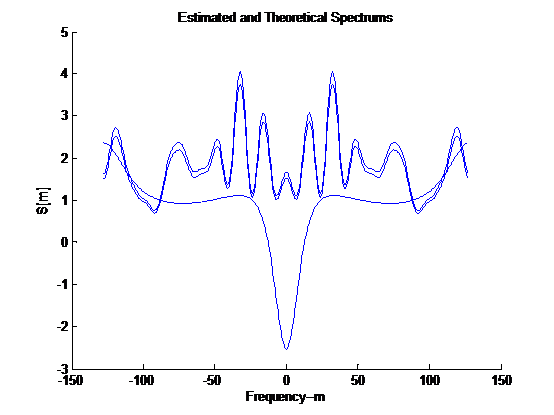
** Figure 5
Tukey
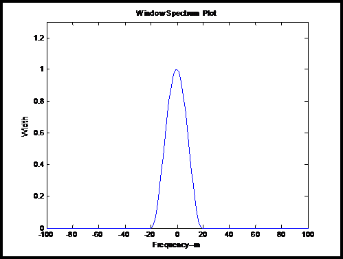
Figure 6
Tukey
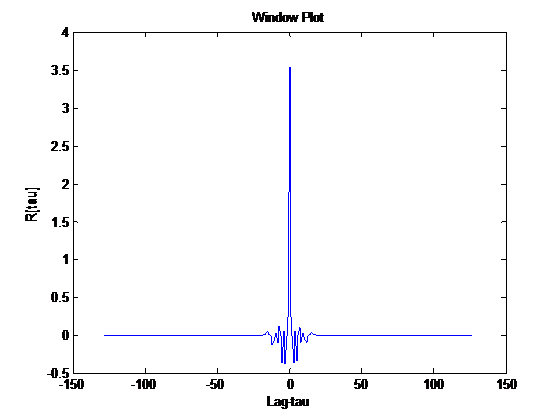
Figure 7
Tukey
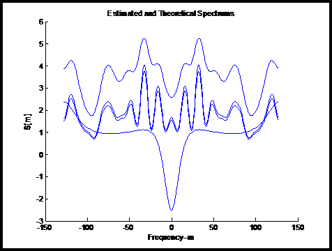
** Figure 5
Blackman
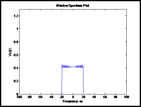
Figure 6
Blackman
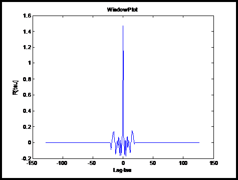
Figure 7
Blackman
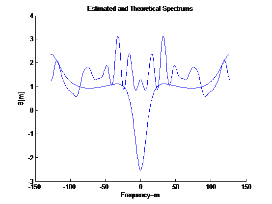
|
Politica de confidentialitate | Termeni si conditii de utilizare |

Vizualizari: 451
Importanta: ![]()
Termeni si conditii de utilizare | Contact
© SCRIGROUP 2025 . All rights reserved