| CATEGORII DOCUMENTE |
| Bulgara | Ceha slovaca | Croata | Engleza | Estona | Finlandeza | Franceza |
| Germana | Italiana | Letona | Lituaniana | Maghiara | Olandeza | Poloneza |
| Sarba | Slovena | Spaniola | Suedeza | Turca | Ucraineana |
1. Theoretical Background
The problems comprised in this chapter are in exclusivity concerned with the investigation of the stress distribution on the cross-section of the plane linear beam subjected to bending. By definition, bending is a deformation suffered by a plane linear beam when loaded with transversal loads.
A number of important assumptions are made:
(a) the beam has a constant cross-section along the entire length of the beam;
(b) the material is isotropic along the entire length of the beam;
(c) the cross-section is characterized by an axis of symmetry;
(d) the transversal loads are acting in the plane of symmetry;
(e) the cross-section remain plane and perpendicular to the deflection curve after the deformation (the Bernoulli-Euler hypothesis).
Note: These assumptions are restricting somehow the generality of the theoretical frame, but the majority of the beams encountered in the structural engineering practice are complying with these limitations.
Consider a local coordinate system Oxyz attached to the left end point of the beam and the axis Oy as the symmetry axis of the cross-section. The transversal loads are also acting in the vertical plan of symmetry Oxy and, consequently, induce into the cross-section of the beam, located at distance x from the origin coordinate system, only two cross-sectional resultants. These are the vertical shear force Vy(x) and the bending moment about the Oz axis Mz(x). The bending moment Mz(x) and shear force Vy(x) conduct to the existence on the cross-section of two stresses: the normal stress sx and shear stress txy. In general both cross-sectional resultants, the vertical shear force and the bending moment, are present on the cross-section. They are not independent functions, being interrelated through the differential relation expressed in chapter 3 of the volume I (the shear force is the first derivative of the bending moment in report to variable x). The cross-section is subjected to non-uniform bending. If the shear force Vy(x) is absent from the cross-section (Vy(x)=0), then the bending moment is constant (Mz(x)=constant) and the cross-section is subjected to pure bending.
Due to the existence of the symmetry plane Oxy for the beam and the definition of the transversal loads in this plane, the deformation of the beam takes place in the same plane. As the result of the deformation of the beam some of the longitudinal fibers are shortened and some are lengthen. Consequently, there are a number of fibers which conserve their length. These fibers constitute the neutral plane and its intersection with the plane of symmetry Oxy defines the deflection curve.
A complete theoretical discussion of the phenomena induced by bending is found in the chapter 7 of the textbook entitled Lectures in Mechanics of Materials. In this chapter only the practical aspect of the application of the formulae related to the normal and shear stress distributions on the cross-sections are discussed.
1.1 The distribution of the normal stress sx (the Naviers Formula)
The cross-sectional resultants are related to the stresses through the following integral relations:
![]() (1)
(1)
![]() (2)
(2)
2. Solved Problems
Problem 2.1
The cantilever beam, shown in Figure 2.1, is subjected to a concentrated moment
![]() acting at the free
end. The cross-section has a square shape with an edge length d = 120 mm. Assuming that the length of the cantilever is
L = 5 m, calculate the following: (a)
the internal resultants diagrams (draw them), (b) the radius of curvature for
the beam, (c) the strain and stress distribution and (d) the maximum
displacement.
acting at the free
end. The cross-section has a square shape with an edge length d = 120 mm. Assuming that the length of the cantilever is
L = 5 m, calculate the following: (a)
the internal resultants diagrams (draw them), (b) the radius of curvature for
the beam, (c) the strain and stress distribution and (d) the maximum
displacement.
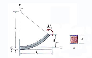
Figure 2.1
A. General Observations
A.1 The cantilever is subjected to pure bending conditions. Consequently the Naviers formula is applied.
A.2 Numerical Application
![]() - the bending moment
- the bending moment
![]() - cantilever length
- cantilever length
![]() - edge length
- edge length
![]() - modulus of elasticity
- modulus of elasticity
B. Calculations
B.1 Reactions Calculation (see Figure 2.1.a)
The reactions, ![]() and
and ![]() , are obtained using the following two equilibrium
equations:
, are obtained using the following two equilibrium
equations:
![]()
![]()
![]()
![]()
![]()
![]()
Solving the above equilibrium equations the reactions are:
![]()
![]()
B.2 Calculation of the Cross-Sectional Resultants (see Figure 2.1.a)
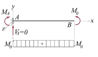
Figure 2.1.a
The
cross-sectional resultants, the shear force ![]() and
bending moment
and
bending moment![]() , on a particular cross-section, located at x distance from end A representing the
origin of the coordinate system, are:
, on a particular cross-section, located at x distance from end A representing the
origin of the coordinate system, are:
![]()
![]()
![]()
![]()
The moment diagram, the only one different than zero, is shown in Figure 2.1.a
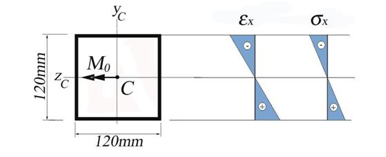
Figure 2.1.b
B.3 Calculation of the Radius of Curvature
The radius of
curvature ![]() is
calculated using the following formula:
is
calculated using the following formula:

where: ![]() is the
moment of inertia about the central axis z.
is the
moment of inertia about the central axis z.
The central moment of inertia is calculated:

![]()
![]()
The radius of curvature ![]() is then
obtained as:
is then
obtained as:

![]()
![]()
Note: the
radius of curvature ![]() is
constant. It can be concluded that when the beam is in a pure bending condition the radius of curvature is always constant
and the defection curve is a circle.
is
constant. It can be concluded that when the beam is in a pure bending condition the radius of curvature is always constant
and the defection curve is a circle.
The curvature ![]() is:
is:
![]()
![]()
![]()
B.4 The Stress and Strain Distributions (see Figure 2.1.b)
The stress and strain distributions are identical in all cross-sections and are shown in Figure 2.1.b. The stress distribution is obtained using the following formula (Naviers Formula):

The distribution of the stress in the cross-section is linear and only the values at the points
located at ![]() and
and ![]() are
necessary to be calculated:
are
necessary to be calculated:
![]()
![]()
![]()
![]()
![]()
![]()
The corresponding maximum normal stresses ![]() and
and ![]() are
obtained:
are
obtained:

![]()
![]()

![]()
![]()
Note: (a)
It is obvious that the maximum normal stresses ![]() and
and ![]() are equal
in the absolute value because the distances from the centroid are equal. When
the cross-section is also symmetrical against the Zc axis only one value is
necessary to be calculated;
are equal
in the absolute value because the distances from the centroid are equal. When
the cross-section is also symmetrical against the Zc axis only one value is
necessary to be calculated;
(b) the area above and below the neutral axis CZc are in compression and tension, respectively.
The linear strain distribution is calculated as:

![]()
![]()

![]()
![]()
Alternatively, the strain distribution on the cross-section using the following formula:
![]()
The normal strains are:
![]()
![]()
![]()
![]()
![]()
![]()
B.5 Calculation of Maximum Displacement
Because the bending moment is known and constant the second-order differential equation of the deflection curve is used:

By integration the slope ![]() and the vertical displacement
and the vertical displacement ![]() are obtained as:
are obtained as:


where ![]() and
and ![]() are
integration constants, which are calculated from the boundary conditions
imposed at
are
integration constants, which are calculated from the boundary conditions
imposed at ![]() :
:
![]()
![]()
![]()
![]()
![]()
![]()
Finally, the expression of the vertical displacement is:

The maximum vertical displacement
![]() is obtained at the cantilever tip
is obtained at the cantilever tip ![]()

![]()

To verify the formula obtained for the vertical
displacement ![]() the MATHCAD
differential equation package is employed. The following is the MATHCAD code:
the MATHCAD
differential equation package is employed. The following is the MATHCAD code:
![]()
![]()

![]()
![]()
![]()
The function ![]() is
plotted in the following sketch.
is
plotted in the following sketch.
The maximum value ![]() read
from the graph is:
read
from the graph is:
![]()
![]()
![]()
Problem 2.2
The aluminum part with a cross-section as illustrated in Figure 2.2 is
subjected to pure bending. Conduct the following tasks: (a) calculate the
maximum bending moment ![]() applied to the member
if the allowable flexural stresses in tension and compression are sall_tens
= 200 MPa and sall_compr = 100 MPa, respectively, and (b) draw
the flexural stress and strain distributions on the cross-section corresponding
to the bending moment determined at point (a).
applied to the member
if the allowable flexural stresses in tension and compression are sall_tens
= 200 MPa and sall_compr = 100 MPa, respectively, and (b) draw
the flexural stress and strain distributions on the cross-section corresponding
to the bending moment determined at point (a).
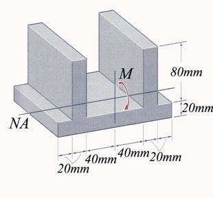
Figure 2.2
A. General Observations
A.1 The cross-section is subjected to pure bending, but a special attention should be given to the fact that the material has different normal allowable stresses.
A.2 Numerical Application
material data
![]() - allowable normal tensile stress
- allowable normal tensile stress
![]() - allowable compressive tensile stress
- allowable compressive tensile stress
![]() - modulus of elasticity
- modulus of elasticity
cross-sectional dimensions
![]() -
web height
-
web height
![]() -
web thickness
-
web thickness
![]() -
flange width
-
flange width
![]() -
flange thickness
-
flange thickness
![]() -
interior distance between webs
-
interior distance between webs
B. Calculations
B.1 Calculation of Cross-section Geometrical Characteristics (see Figure 2.2.a)
Note: All calculations related to the cross-sectional characteristics are conducted in cm.
The cross-section is considered composed from three individual shapes: two webs and a flange. The areas of the web, flange and the total area of the cross-section are calculated as:
![]()
![]()
![]() - the web area
- the web area
![]()
![]()
![]() - the flange area
- the flange area
![]()
![]()
![]()
The
centroid is located on the axis of symmetry
and consequently, only the vertical position is necessary to be calculated.
The initial coordinate system OYZ is
considered located at the level of the centroid of the webs. The vertical
position ![]() of the cross-sectional centroid is obtained:
of the cross-sectional centroid is obtained:

![]()
![]()
where ![]() -
distance from O to the web centroid
-
distance from O to the web centroid

![]()
![]() -
distance from O to the flange centroid
-
distance from O to the flange centroid
The moment of
inertia of the entire cross-section against the CZc axis ![]() is obtained:
is obtained:


![]()
where:
![]()
![]()
![]() -
distance from C to the web centroid
-
distance from C to the web centroid
![]()
![]()
![]() - distance from C to the flange centroid
- distance from C to the flange centroid
The section modulus is calculated as follows:
![]()
where:

![]()
![]() - for the superior fiber
- for the superior fiber

![]()
![]()

![]()
![]() - for the inferior fiber
- for the inferior fiber

![]()
![]()
Then, the section modulus ![]() is:
is:
![]()
![]()
![]()
B.2 Calculation of the Capable Bending Moment
Due to the fact that the material considered has different allowable normal stress in tension and compression the calculation has to identify the maximum tensile and compressive normal stress existing on the cross-section. The bending moment M indicated in Figure 2.2 is negative and consequently, the area located above the neutral axis (CZc axis) is in tension, while the area located below is in compression.
The verification formulas are:
 - for the tensile normal stress area
 - for the compressive normal stress area
The unknown values of the corresponding bending moments are:
![]()
![]()
![]()
![]()
![]()
![]()
The capable
bending moment ![]() characterizing the entire cross-section is:
characterizing the entire cross-section is:
![]()
![]()
![]()
Note: The compressive allowable compressive stress is reached first.
B.3 Normal Stess and Strain Diagrams (see Figure 2.2.a)
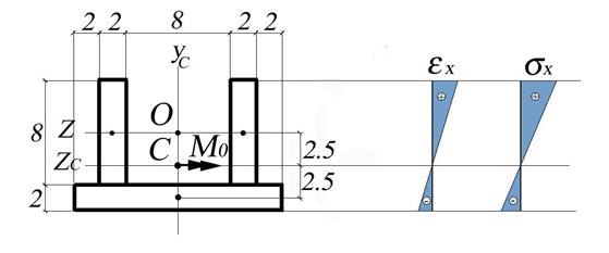
Figure 2.2.a
The real distribution of the normal stress on the
cross-section corresponding to the bending moment ![]() is obtained:
is obtained:

![]()
![]()

![]()
![]()
The corresponding normal strains are calculated as:

![]()
![]()

![]()
![]()
The final stress and strain distributions are plotted in Figure 2.2.a.
Problem 2.3 The timber beam made of four planks tied together with screws to form a box section, as shown in Figure 2.3, is subjected to pure bending. If the flexural stress at point B of the cross section is a 6.2 MPa tensional stress, determine (a) the bending stress and strain distribution on the cross-section, (b) the bending moment carried by the cross-section, (c) the flexural stresses at points A and D of the cross-section, (d) the axial force acting on the top and bottom planks and (e) the capable bending moment of the cross-section considering that the wood has allowable flexural stresses in tension and compression sall_tens =30 MPa and sall_compr =20 MPa.
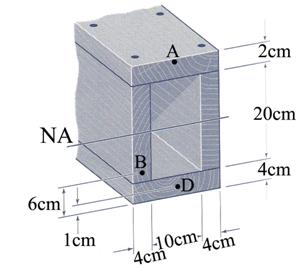
Figure 2.3
A. General Observations
A.1 The cross-section is subjected to pure bending, but a special attention should be given to the fact that the material has different normal allowable stresses.
A.2 Numerical Application
material data
![]() - allowable normal tensile stress
- allowable normal tensile stress
![]() - allowable compressive tensile stress
- allowable compressive tensile stress
![]() - modulus of elasticity
- modulus of elasticity
cross-sectional dimensions
![]() -
web height
-
web height
![]() -
web thickness
-
web thickness
![]() -
flange width
-
flange width
![]() -
top flange thickness
-
top flange thickness
![]() -
bottom flange thickness
-
bottom flange thickness
point B and D
![]() -
distance measured from the bottom of the box beam
-
distance measured from the bottom of the box beam
![]() -
effective normal stress at point B
-
effective normal stress at point B
![]() - distance measured from the bottom of the box
beam
- distance measured from the bottom of the box
beam
B. Calculations
B.1 Calculation of the Cross- Section Geometrical Characteristics (see Figure 2.3.a)
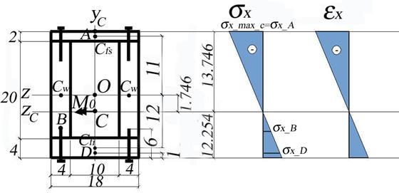
Figure 2.3.a
The cross- section is composed from four rectangles: top flange, two webs and bottom flange. The corresponding areas of the components and the total area of the cross-section are calculated:
Note: All dimensions used in the calculations of the cross-section geometrical characteristics are in cm.
![]()
![]()
![]() -
area of the web
-
area of the web
![]()
![]()
![]() -
area of the top flange
-
area of the top flange
![]()
![]()
![]() -
area of the bottom flange
-
area of the bottom flange
![]()
![]()
![]() -
total area
-
total area
The cross- section is symmetric against the vertical axis OYc and consequently, only the vertical position of the cross- section centroid is required to be calculated. The general coordinate system OYcZ is anchored in the centroid of the webs.
![]() -
distance from the point O to the web
centroid.
-
distance from the point O to the web
centroid.

![]()
![]() - distance from the point O to the top flange centroid.
- distance from the point O to the top flange centroid.

![]()
![]() - distance from the point O to the botom flange centroid
- distance from the point O to the botom flange centroid

![]()
![]()
the vertical position of the centroid
Note: The neutral axis, NA, is identical to the central horizontal axis of the coordinate system CYcZc.
The new coordinate system CYcZc is moved in the centroid C of the cross- section. The moments of inertia, Izc, of the entire cross- section calculated against the axis CZc is obtained:
![]()
![]()
![]() - distance from the point C to the web centroid.
- distance from the point C to the web centroid.
![]()
![]()
![]() - distance from the point C to the top flange centroid.
- distance from the point C to the top flange centroid.
![]()
![]()
![]() - distance from the point C to the botom flange centroid
- distance from the point C to the botom flange centroid


![]() -
cross- section moment of inertia
-
cross- section moment of inertia
The section modulus W is obtained:

![]()
![]() - distance from NA to the upper edge of the top flange
- distance from NA to the upper edge of the top flange

![]()
![]() - distance from NA to the lower edge of the bottom flange
- distance from NA to the lower edge of the bottom flange

![]()

![]()
![]()
![]()
![]()
- sectional modulus
B.2
Accordingly to
the Naviers Formula the normal
stress distribution on the cross- section is linear. To draw the diagram, two
point are necessary: the first point is the centroid and the second is the
given normal stress ![]() at
point B. The resulting diagram of the normal stress is shown in Figure 2.3.a.
The maximum values of the normal stresses,
at
point B. The resulting diagram of the normal stress is shown in Figure 2.3.a.
The maximum values of the normal stresses, ![]() and
and ![]() , corresponding to the upper edge of the top flange and the
lower edge of the bottom flange, respectively, are calculated using simple
geometrical proportions.
, corresponding to the upper edge of the top flange and the
lower edge of the bottom flange, respectively, are calculated using simple
geometrical proportions.

![]()
![]()

![]()
![]()
where ![]() is the distance
measured from the neutral axis, NA,
to point B.
is the distance
measured from the neutral axis, NA,
to point B.

![]()
![]()
The
corresponding maximum strains, ![]() and
and ![]() calculated at the
upper edge of the top flange and the lower edge of the bottom flange,
respectively, are obtained as:
calculated at the
upper edge of the top flange and the lower edge of the bottom flange,
respectively, are obtained as:

![]()
![]()

![]()
![]()
Note: The values of the obtained maximum normal stresses and corresponding strains indicate that the area above the neutral axis is in compression, while the area below the neutral axis is in tension.
B.3 Calculation of the Bending Moment
The bending moment, Mo, acting on the CZc axis and corresponding to the normal stress distribution calculated in section B.2 is obtained:

![]()
![]()
Note: Due to the rounded to the third decimal of the numbers used in the manual calculation an insignificant numerical error appears in comparison with similar MATHCAD results.
To verify the maximum values of the normal stresses diagram, calculated in section B.2, these values are recalculated using the moment Mo and Naviers Formula:

![]()
![]()

![]()
![]()
B.4 Calculation of Normal Stress at points A and D
The normal stresses at points A and D can be calculated using two methods: (a) Naviers Formula or (b) geometrical proportions of the linear diagram shown in Figure 2.3.a.
(a) Naviers Formula

![]()
![]()

![]()
![]()
where: 
![]()
![]()
![]()
![]()
![]()
(b) Geometrical Method
![]()
![]()
![]()

![]()
![]()
B.4 Calculation of the Axial Forces of the Flanges
The axial forces in the flanges are obtained using the normal stress diagram shown in Figure 2.3.b.
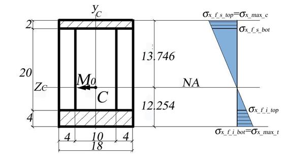
Figure 2.3.b.
(a) The axial force in the top flange
![]()
![]()
![]()
![]()
![]()
![]()

![]()
![]()
![]()
![]()
![]()
(b) The axial force in the bottom flange
![]()
![]()
![]()

![]()
![]()
![]()
![]()
![]()
![]()
![]()
![]()
B.5 Calculation of the Capable Bending Moment
In the previous
sections the sign of the bending moment Mo
is positive, as shown in Figure 2.3.b, being established by the sign of the
normal stress ![]() imposed at point B.
The calculation of the capable bending moment pertinent to the entire
cross-section, subjected to pure bending against the central axis CZc, requires the examination of both
conditions, positive and negative directions of the bending moment.
imposed at point B.
The calculation of the capable bending moment pertinent to the entire
cross-section, subjected to pure bending against the central axis CZc, requires the examination of both
conditions, positive and negative directions of the bending moment.
(a)
If ![]() >0
>0
The verification formulas corresponding to the extreme fibers are:


The capable bending moment calculated under the assumption that the bending moment is positive, a vector parallel with the positive CZc axis, is:
![]()
![]()
![]()
(b) If ![]() <0
<0
The verification formulas corresponding to the extreme fibers are:


The capable bending moment calculated under the assumption that the bending moment is negative, a vector parallel with the negative CZc axis, is:
![]()
![]()
![]()
The capable bending moment of the entire cross-section is obtained as:
![]()
![]()
![]()
![]()
![]()
![]()
![]()
Problem 2.4
For the cross- section shown in Figure 2.4, considered subjected to a non-uniform
bending characterized by a bending moment Mo=55
kNm and shear force Vo=10 kN,
conduct the following tasks: (a) calculate the normal stress distribution on
the cross- section, (b) calculate the shear stress distribution on the cross-
section and (c) verify the cross- section, considering ![]() and
and ![]() .
.
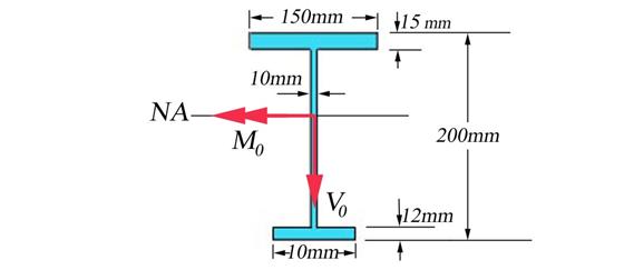
Figure 2.4
A. General Observations
A.1 The cross-section is subjected to non-uniform bending. Both Naviers and Jourawskis Formulas are applicable. The beam is made of steel and consequently, the allowable bending stress has an equal value for both tensile and compressive normal stress.
A.2 Numerical Application
cross- sectional resultants
![]() - bending moment
- bending moment
![]() - shear force
- shear force
material data
 - allowable normal tensile and
compressive stress
- allowable normal tensile and
compressive stress
![]() - allowable shear stress
- allowable shear stress
![]() - modulus of elasticity
- modulus of elasticity
cross-sectional dimensions
![]()
![]()
![]()
![]()
![]()
![]()
![]()
![]()
![]() - section height
- section height
![]()
![]()
![]() - web thickness
- web thickness
![]()
![]()
![]() - top flange width
- top flange width
![]()
![]()
![]() - bottom flange width
- bottom flange width
![]()
![]()
![]() - top flange thickness
- top flange thickness
![]()
![]()
![]() - bottom flange thickness
- bottom flange thickness
![]()
![]()
![]() -
web height
-
web height
B. Calculations
B.1 Calculation of the Cross- Section Geometrical Characteristics (see Figure 2.4.a)
The cross- section consists on three individual rectangular areas: upper and lower flanges and the web. The corresponding areas are calculated:
![]()
![]()
 -
area of the top flange
-
area of the top flange
![]()
![]()
![]() -
area of the bottom flange
-
area of the bottom flange
![]()
![]()
![]() -
area of the web
-
area of the web
![]()
![]()
![]() -
total area
-
total area
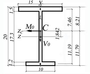
Figure 2.4.a
The initial coordinate system OYcZ passes through the centroid of the web. The distances from point O to the lower and upper flange centroids are obtained:
![]()
![]()
![]()
![]() distance from the point O to the upper flange centroid.
distance from the point O to the upper flange centroid.
![]()
![]()
![]() distance from the point O to the lower flange centroid.
distance from the point O to the lower flange centroid.

![]()
![]()
Note: The neutral axis, NA, is identical to the central horizontal axis of the coordinate system CYcZc.
The new coordinate system CYcZc is moved in the centroid C of the cross- section. The moments of inertia, Izc, of the entire cross- section calculated against the axis CZc is obtained:
![]()
![]()
![]()
![]()
![]()
![]()
![]()
![]()
![]()


![]()
The sectional modulus of the cross- section is obtained as:
![]()
![]()
![]() - distance from NA to the upper edge of the top flange
- distance from NA to the upper edge of the top flange
![]()
![]()
![]() - distance from NA to the lower edge of the bottom flange
- distance from NA to the lower edge of the bottom flange


![]()


![]()
![]()
![]()
![]()
-sectional modulus
B.2 Calculation
of the ![]() Diagram)
Diagram)
The stress distribution is obtained using the following formula (Naviers Formula):

The maximum
values of the normal stresses, ![]() and
and ![]() , corresponding to the upper edge of the top flange and the
lower edge of the bottom flange, respectively, are calculated:
, corresponding to the upper edge of the top flange and the
lower edge of the bottom flange, respectively, are calculated:

![]()
![]()

![]()
![]()
The corresponding strains are obtained:

![]()
![]()

![]()
![]()
The stress and strain distributions are shown in Figure 2.4.b.
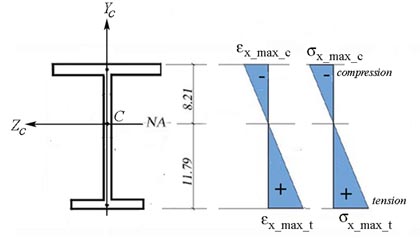
Figure 2.4.b
B.3 Calculation of Shear Stress Distribution (t Diagram)
The shear flow and stress diagram is calculated employing the Jurawskis Formula detailed in the theoretical paragraph of the chapter. The cross-section is divided into four distinct rectangular areas, A1 through A4, where the Jurawskis formula is applicable. This division is shown in Figure 2.4.c.
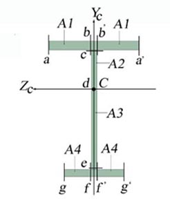
Figure 2.4.c
Each area is delineated by two cuts (A1:a-b or a-b, A2:c-d or c-d, A3:e-f and A4:g-f or g-f). The variation of the corresponding shear stress is calculated on each of the four areas.
B.3.a Upper
Flange (![]() shear stress)
shear stress)
The horizontal cut 1-1 is made, as shown in Figure 2.4.d, at distance s1 measured from a and increasing towards b.
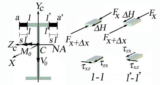
Figure 2.4.d
Theoretical rational:
![]()
![]()
![]() (area above the NA is
in compression).
(area above the NA is
in compression).
![]()
![]()
![]()
![]()
![]()
![]()
![]()
![]()
![]()
![]()
![]()
![]()
![]()
![]()
![]()
![]()
![]()
![]()
![]()
Numerical calculations:
![]()
![]()
![]() -
thickness of the cut at s1
-
thickness of the cut at s1
 -
static moment about the neutral axis
-
static moment about the neutral axis
 -
shear flow on the cut area
-
shear flow on the cut area
 -
shear stress on the cut area
-
shear stress on the cut area
The above
functions are particularized for the two limiting cuts of the segment ab. Only two values are sufficient because the
variation of the shear stress ![]() is linear.
is linear.
cut a
![]()
![]()
![]()
![]()
![]()
![]()
![]()
- shear stress at the face of the flange
cut b

![]()
![]()
![]()
![]()
![]()
![]()
![]()
![]()
- shear stress at the face of the web
The above
calculations refer only to the left area of the upper flange. Due to the
symmetry exhibit by the upper flange against the CYc axis, the shear stress ![]() calculated for the
left side of the upper flange is symmetric with the shear stress on the right
side.
calculated for the
left side of the upper flange is symmetric with the shear stress on the right
side.
B.3.b Lower
Flange (![]() shear stress)
shear stress)
The calculation
of the shear stress ![]() corresponding to the
lower flange is conducted in a similar manner with the calculation developed in
section B.3.a. The horizontal cut 3-3 is
made, as shown in Figure 2.4.e, at
distance s3 measured from g and increasing towards f.
corresponding to the
lower flange is conducted in a similar manner with the calculation developed in
section B.3.a. The horizontal cut 3-3 is
made, as shown in Figure 2.4.e, at
distance s3 measured from g and increasing towards f.
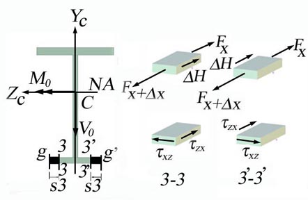
Figure 2.4.e
Theoretical rational:
![]()
![]()
![]() (area below the NA is
in tension)
(area below the NA is
in tension)
![]()
![]()
![]()
![]()
![]()
![]()
![]()
![]()
![]()
![]()
![]()
![]()
![]()
![]()
![]()
![]()
![]()
![]()
![]()
Numerical calculations:
![]()
![]()
![]() -
thickness of the cut at s3
-
thickness of the cut at s3
 -
static moment about the neutral axis
-
static moment about the neutral axis
 -
shear flow on the cut area
-
shear flow on the cut area
 -
shear stress on the cut area
-
shear stress on the cut area
The above
functions are particularized for the two limiting cuts of the segment gf. Only two values are sufficient because the
variation of the shear stress ![]() is linear.
is linear.
cut g
![]()
![]()
![]()
![]()
![]()
![]()
![]()
- shear stress at the face of the flange
cut f

![]()
![]()
![]()
![]()
![]()
![]()
![]()
![]()
- shear stress at the face of the web
The above
calculations refer only to the left area of the upper flange. Due to the
symmetry exhibit by the upper flange against the CYc axis, the shear stress ![]() calculated for the
left side of the lower flange is symmetric with the shear stress on the right
side.
calculated for the
left side of the lower flange is symmetric with the shear stress on the right
side.
B.3.c Web (![]() shear stress)
shear stress)
The calculation
of the shear stress ![]() on the area of the web
located above the neutral axis, area A2, is conducted by considering the
equilibrium of the infinitesimal three-dimensional body as shown in Figure 2.4.f.
The horizontal cut 2-2 is made at
distance s2 measured from c and increasing towards d.
on the area of the web
located above the neutral axis, area A2, is conducted by considering the
equilibrium of the infinitesimal three-dimensional body as shown in Figure 2.4.f.
The horizontal cut 2-2 is made at
distance s2 measured from c and increasing towards d.
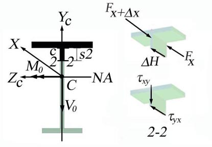
Figure 2.4.f
Theoretical rational:
![]()
![]()
![]() (area above the NA is
in compression).
(area above the NA is
in compression).
![]()
![]()
![]()
![]()
![]()
![]()
![]()
![]()
![]()
![]()
![]()
![]()
![]()
![]()
![]()
![]()
![]()
![]()
![]()
Numerical calculations:
![]()
![]()
![]() -
thickness of the cut at s3
-
thickness of the cut at s3

- static moment about the neutral axis
 -
shear flow on the cut area
-
shear flow on the cut area
 -
shear stress on the cut area
-
shear stress on the cut area
The variation of the shear stress is a second- order parabola. Only two values of the shear stress are necessary and they are calculated at the location of the junction between the upper flange and the web and at the neutral axis location.
cut c
![]()
![]()
![]()
![]()
![]()
![]()
![]()
- shear stress at the junction between upper flange and web
cut d
![]()
![]()
![]()
![]()
![]()
![]()
![]()
![]()
![]()
shear stress at the neutral axis
The variation of
the shear stress ![]() on the area below the
neutral axis, shown in Figure 2.4.g, is parametrically calculated using the
following rational:
on the area below the
neutral axis, shown in Figure 2.4.g, is parametrically calculated using the
following rational:
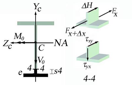
Figure 2.4.g
Theoretical rational:
![]()
![]()
![]() (area below the NA is
in tension).
(area below the NA is
in tension).
![]()
![]()
![]()
![]()
![]()
![]()
![]()
![]()
![]()
![]()
![]()
![]()
![]()
![]()
![]()
![]()
![]()
![]()
![]()
Numerical calculations:
![]()
![]()
![]() -
thickness of the cut at s3
-
thickness of the cut at s3

- static moment about the neutral axis
 -
shear flow on the cut area
-
shear flow on the cut area
 -
shear stress on the cut area
-
shear stress on the cut area
The variation of the shear stress is a second- order parabola. Only two values of the shear stress are necessary to be calculated and they are expressed at the location of the junction between the lower flange and the web and at the neutral axis location.
cut e
![]()
![]()
![]()
![]()
![]()
![]()
![]()
- shear stress at the junction between lower flange and web
cut d
![]()
![]()
![]()
![]()
![]()
![]()
![]()
![]()
![]()
- shear stress at the neutral axis
The shear stress distribution on the entire cross-section, calculated above, is shown in Figure 2.4.h.
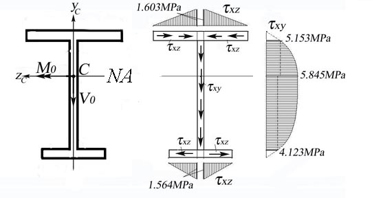
Figure 2.4.h
B.4 Verification of the Cross-Section
B.4.a
Verification of the
The verification of the cross-section is conducted considering the following formula:
![]()
![]()
![]()
![]()
B.4.b Verification of the Shear Stress
The verification of the cross-section is conducted considering the following formula:
![]()
where:
![]()
![]()
![]()
![]()
- maximum shear stress on the web
![]()
B.5 The Web Shear Force
The shear force carried
by the web is obtained by integrating on the web thickness the ![]() shear stress diagram
pictured in Figure 2.4.h:
shear stress diagram
pictured in Figure 2.4.h:
![]() - the shear force in the web of the
cross- section
- the shear force in the web of the
cross- section
where:
![]()
![]()
![]()
![]()
![]()
![]()
The ratio between the web shear force and the total shear force acting on the cross- section is:
![]()

The ratio indicates that the web transfers 93% of the total shear force acting on the cross-section. For this reason the codes employed for the calculations of steel structures are imposing that the entire shear force to be transferred only to the web.
Then, the average shear stress in the web is:

![]()
![]()
Problem 2.5
For the cross- section shown in Figure 2.5, considered subjected to a
non-uniform bending characterized by a bending moment Mo and shear force Vo=50 kN,
conduct the following tasks: (a) calculate the bending capacity and normal
stress distribution on the cross- section, (b) calculate the shear stress
distribution on the cross- section and verify the cross- section,
considering ![]() and
and ![]() .
.
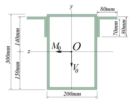
Figure 2.5
A. General Observations
A.1 The cross-section is subjected to non-uniform bending. Both Naviers and Jourawskis Formulas are applicable. The beam is made of steel and consequently, the allowable bending stress has an equal value for both tensile and compressive normal stress.
The shear stress induced by the existence of the shear force Vo is calculated using the observation that for a thin- wall closed cross- section the shear flow is null in the axis of symmetry of the cross- section.
A.2 Numerical Application
cross- sectional resultants
![]() - shear force
- shear force
material data
![]() - allowable normal tensile and
compressive stress
- allowable normal tensile and
compressive stress
![]() - allowable shear stress
- allowable shear stress
![]() - modulus of elasticity
- modulus of elasticity
cross-sectional dimensions
![]() - tubular cross- section width
- tubular cross- section width
![]() - tubular cross- section height
- tubular cross- section height
![]() - tubular cross- section thickness
- tubular cross- section thickness
![]() - equal legs L shape width
- equal legs L shape width
![]() - L shape thickness
- L shape thickness
![]() -
position of the L shape (see Figure 2.5)
-
position of the L shape (see Figure 2.5)
B. Calculations
B.1 Calculation of the Cross- Section Geometrical Characteristics
The cross- section consists on three individual areas: a tubular cross-section and two equal legs L shapes. Their corresponding geometrical characteristics are calculated as shown below.
B.1.1 Calculation of the L Shape Geometrical Characteristics (see fig. 2.5.a)
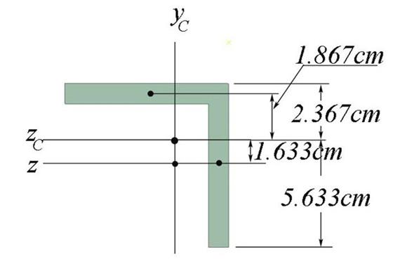
Figure 2.5.a
![]()
![]()
![]()
![]()
![]()
![]()
![]()
![]()
![]() -
area of the L shape
-
area of the L shape

![]()
![]() - distance from the point O to the upper flange centroid.
- distance from the point O to the upper flange centroid.
![]() -
distance from the point O to the
lateral flange centroid.
-
distance from the point O to the
lateral flange centroid.

![]()
![]()
![]()
![]()
![]() - distance from the point C to the upper flange centroid.
- distance from the point C to the upper flange centroid.
![]()

![]() -
distance from the point
-
distance from the point
C to the upper flange centroid.


![]() - moment of inertia of the L shape computed
with respect to its local centroid
- moment of inertia of the L shape computed
with respect to its local centroid

![]()
![]() -
eccentricity of L shape
-
eccentricity of L shape
![]()
![]()
![]()
B.1.2 Calculation of the Tubular Cross- Section Geometrical Characteristics (see fig. 2.5.b)
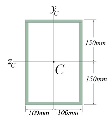
Figure 2.5.b
![]()
![]()
![]() -
area of the exterior rectangle
-
area of the exterior rectangle
![]()
![]()
 -
area of the exterior rectangle
-
area of the exterior rectangle
![]()
![]()
![]() -
area of the tubular cross- section
-
area of the tubular cross- section

![]()
![]()
- moment of inertia of the tubular cross- section
B.1.3 Calculation of the Cross- Section Geometrical Characteristics (see fig. 2.5.c)
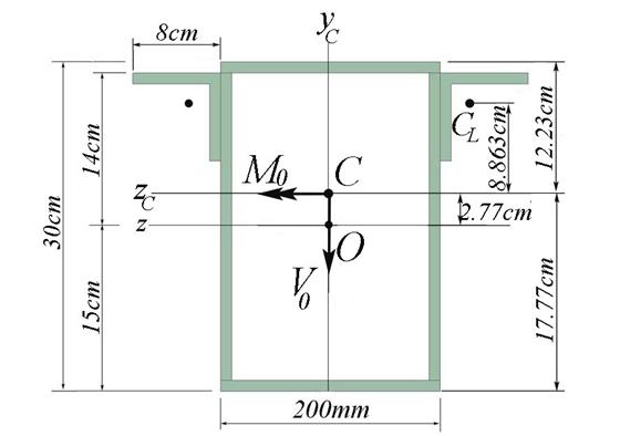
Figure 2.5.c
![]()
![]()
![]() -
total area
-
total area
The initial coordinate system OYcZ passes through the centroid of the web. The distances from point O to the lower and upper flange centroids are obtained:
![]()

![]()
![]() - distance from the point O to the center of the L shape
- distance from the point O to the center of the L shape

![]()
![]() -
centroid of the cross- section
-
centroid of the cross- section
Note: The neutral axis, NA, is identical to the central horizontal axis of the coordinate system CYcZc.
The new coordinate system CYcZc is moved in the centroid C of the cross- section. The moments of inertia, Izc, of the entire cross- section calculated against the axis CZc is obtained:
![]()
![]()
![]() - distance from the point C to the centroid of
the tubular cross- section
- distance from the point C to the centroid of
the tubular cross- section
![]()
![]()
![]() - distance from the point C to the centroid of
the tubular cross- section
- distance from the point C to the centroid of
the tubular cross- section
![]()
![]()
![]()
The sectional modulus of the cross- section is obtained as:

![]()
![]() - distance from NA to the upper edge of cross- section
- distance from NA to the upper edge of cross- section

![]()
![]() - distance from NA to the lower edge of the cross- section
- distance from NA to the lower edge of the cross- section
![]()
![]()
![]()
![]()
![]()
![]()
![]()
-sectional modulus
B.2 Calculation of Bending Capacity and Normal Stress Diagram (see fig. 2.5.d)
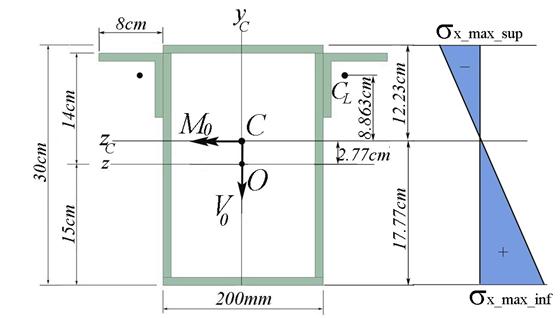
Figure 2.5.d
![]()
![]()
![]()
-capable moment
The stress distribution is obtained using the following formula (Naviers Formula):
The maximum
values of the normal stresses, ![]() and
and ![]() , corresponding to the upper edge of the top flange and the
lower edge of the bottom flange, respectively, are calculated:
, corresponding to the upper edge of the top flange and the
lower edge of the bottom flange, respectively, are calculated:

![]()
![]()

![]()
![]()
B.3 Calculation of Shear Stress Distribution (t Diagram)
The shear flow and stress diagram is calculated employing the Jurawskis Formula detailed in the theoretical paragraph of the chapter. Due to the vertical symmetry of the cross-section, symmetry against the CYc axis, the shear flow at the symmetry locations is zero. Consequently, the calculation of the shear flow is conducted only on the left half of the cross-section, which is divided into six distinct rectangular areas, A1 through A6, where the Jurawskis formula is applicable. This division is shown in Figure 2.5.e. The shear flow on the remaining right half of the cross-section is symmetric.
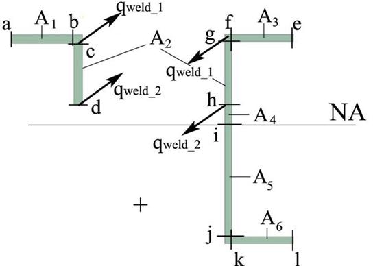
Figure 2.5.e
Each area is delineated by two cuts (A1:a-b, A2:c-d, A3:e-f, A4:d-i, A5:i-j and A6:k-l). The cuts c and d intersects the thicknesses of two bodies (L shape flange and tubular section web) resulting in a violation of the Juravskis Formula assumption of the constant distribution through thickness. This assumption is impossible to be made in this case due to existence of two thicknesses. A separation of the L shape and the tubular cross- section is required and application of the Juravskis Formula is conducted for each one of them. For clarity the cuts c and d are retained only for the L shape, while for the tubular cross- section they are renamed g and h.
Note: It has to be emphasized that the separation of the original cross- section into L shape and tubular cross- section requires the calculations of the shear flow in the welds.
B.3.a Calculation of the Shear Flow in Welds (see Figure 2.5.f )
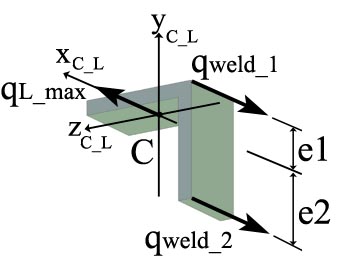
Figure 2.5.f
The total shear in the L shape is calculated as:

![]()
![]()
where ![]()
![]()
![]()
To calculate the shear flow in the welds two equilibrium equations are used:
 -
projections on x axis
-
projections on x axis
 -
moment about z axis passing through the L shape centroid
-
moment about z axis passing through the L shape centroid
Explicitly the two equations, containing the shear flow in the welds as unknown quantities are written as:
![]()
![]()

The solutions, representing the shear flow in each weld, are:
![]()
![]()
B.3.b Calculation of the Shear Flow on the L Shape
B.3.b.1
Horizontal Flange (![]() shear stress)
shear stress)
The horizontal cut 1-1 is made, as shown in Figure 2.5.g, at distance s1 measured from a and increasing towards b.
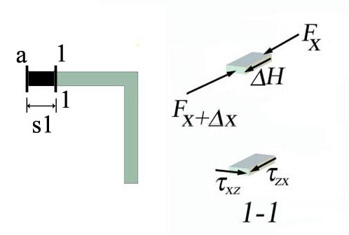
Figure 2.5.g
Theoretical rational:
![]()
![]()
![]() (area above the NA is
in compression).
(area above the NA is
in compression).
![]()
![]()
![]()
![]()
![]()
![]()
![]()
![]()
![]()
![]()
![]()
![]()
![]()
![]()
![]()
![]()
![]()
![]()
![]()
Numerical calculations:
![]()
![]()
![]() -
thickness of the cut at s1
-
thickness of the cut at s1
 -
static moment about the neutral axis
-
static moment about the neutral axis
-
shear flow on the cut area
-
shear stress on the cut area
The above functions are particularized for the two limiting
cuts of the segment ab. Only two values are
sufficient because the variation of the shear stress ![]() is linear.
is linear.
cut a
![]()
![]()
![]()
![]()
![]()
![]()
![]()
- shear stress at the face of the flange
cut b
![]()
![]()
![]()
![]()
![]()
![]()
![]()
![]()
![]()
- shear stress at the face of the web
B.3.b.2 Vertical
Flange (![]() shear stress)
shear stress)
The calculation
of the shear stress ![]() on the area of
vertical flange, area A2, is conducted by considering the equilibrium of the
infinitesimal three-dimensional body as shown in Figure 2.5.h. The horizontal
cut 2-2 is made at distance s2 measured from c and increasing towards d.
on the area of
vertical flange, area A2, is conducted by considering the equilibrium of the
infinitesimal three-dimensional body as shown in Figure 2.5.h. The horizontal
cut 2-2 is made at distance s2 measured from c and increasing towards d.
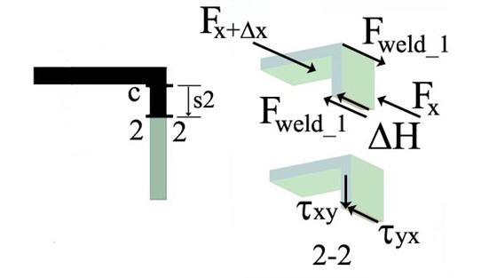
Figure 2.5.h
Theoretical rational:
(a) in the absence of the weld_1
![]()
![]()
![]() (area above the NA is
in compression).
(area above the NA is
in compression).
![]()
![]()
![]()
![]()
![]()
![]()
![]()
![]()
![]()
![]()
![]()
![]()
![]()
![]()
![]()
![]()
![]()
(b) the weld_1 effect:
![]() the reaction induced
by the weld_1 on the cut cross-section is equal and has an opposite direction
the reaction induced
by the weld_1 on the cut cross-section is equal and has an opposite direction ![]()
![]()
![]()
![]()
![]()
(c) the resultant shear stress on the cut cross-section is:
![]()
![]()
![]()
Numerical calculations:
![]()
![]()
![]() -
thickness of the cut at s2
-
thickness of the cut at s2
![]()
static moment about the neutral axis
 -
shear flow on the cut area if the weld wouldnt exist
-
shear flow on the cut area if the weld wouldnt exist
![]() -
shear flow on the cut area
-
shear flow on the cut area
-
shear stress on the cut area
The variation of the shear stress is a
second- order parabola. To draw the variation of the shear stress ![]() three points are
necessary. They are: the cut c, cut d and the location of the cut where the
shear stress is zero.
three points are
necessary. They are: the cut c, cut d and the location of the cut where the
shear stress is zero.
cut c
![]()
![]()
![]()
![]()
![]()
![]()
![]()
![]()
shear stress at the junction between upper flange and web
cut d
![]()
![]()
![]()
![]()
![]()
![]()
![]()
![]()
![]()
![]()
- shear stress at the lower edge of the vertical flange
Note: It
is observed that the shear stress ![]() changes the sign
in-between the cuts c and d. The position of the cut where the
shear stress
changes the sign
in-between the cuts c and d. The position of the cut where the
shear stress ![]() is zero is calculated
from the condition that the shear flow is null on the interval between cuts c and d.
is zero is calculated
from the condition that the shear flow is null on the interval between cuts c and d.
![]()
the position is:
B.3.c Calculation of the Shear Flow on the tubular cross- section
B.3.c.1 Upper
Flange (![]() shear stress)
shear stress)
The horizontal cut 3-3 is made, as shown in Figure 2.5.h, at distance s3 measured from e and increasing towards f.
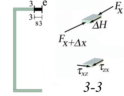
Figure 2.5.i
Theoretical rational:
![]()
![]()
![]() (area above the NA is
in compression).
(area above the NA is
in compression).
![]()
![]()
![]()
![]()
![]()
![]()
![]()
![]()
![]()
![]()
![]()
![]()
![]()
![]()
![]()
![]()
![]()
![]()
![]()
Numerical calculations:
![]()
![]()
![]() -
thickness of the cut at s3
-
thickness of the cut at s3
 -
static moment about the neutral axis
-
static moment about the neutral axis
 -
shear flow on the cut area
-
shear flow on the cut area
 -
shear stress on the cut area
-
shear stress on the cut area
The above functions are particularized for the two limiting
cuts of the segment ef. Only two values are
sufficient because the variation of the shear stress ![]() is linear.
is linear.
cut e
![]()
![]()
![]()
![]()
![]()
![]()
![]()
shear stress at the face of the flange
cut f

![]()
![]()
![]()
![]()
![]()
![]()
![]()
![]()
shear stress at the face of the web
B.3.c.2 The web
(![]() shear stress)
shear stress)
The web of the
tubular cross-section has three distinct areas where the variation of the shear
stress ![]() has
to be determined: area A2, located between the upper flange and the position of
the lower weld, area A4, located between the lower weld and the neutral axis NA
of the entire cross-section, and area A5, located between the neutral axis NA
of the entire cross-section and the lower flange.
has
to be determined: area A2, located between the upper flange and the position of
the lower weld, area A4, located between the lower weld and the neutral axis NA
of the entire cross-section, and area A5, located between the neutral axis NA
of the entire cross-section and the lower flange.
B.3.c.2.a Area A2
The calculation
of the shear stress ![]() on the area of
vertical flange, area A2, is conducted by considering the equilibrium of the
infinitesimal three-dimensional body as shown in Figure 2.5.j. The horizontal
cut 4-4 is made at distance s4 measured from g and increasing towards h.
on the area of
vertical flange, area A2, is conducted by considering the equilibrium of the
infinitesimal three-dimensional body as shown in Figure 2.5.j. The horizontal
cut 4-4 is made at distance s4 measured from g and increasing towards h.
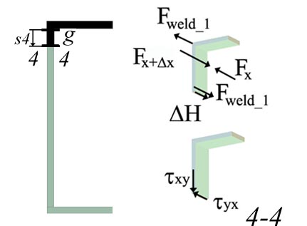
Figure 2.5.j
Theoretical rational:
(a) in the absence of the weld_1
![]()
![]()
![]() (area above the NA is
in compression).
(area above the NA is
in compression).
![]()
![]()
![]()
![]()
![]()
![]()
![]()
![]()
![]()
![]()
![]()
![]()
![]()
![]()
![]()
![]()
![]()
(d) the weld_1 effect:
![]() the reaction induced
by the weld_1 on the cut cross-section is equal and has an opposite direction
the reaction induced
by the weld_1 on the cut cross-section is equal and has an opposite direction ![]()
![]()
![]()
![]()
![]()
(e) the resultant shear stress on the cut cross-section is:
![]()
![]()
![]()
Numerical calculations:
![]()
![]()
![]() -
thickness of the cut at s4
-
thickness of the cut at s4

static moment about the neutral axis
 -
shear flow on the cut area if the weld would not exist.
-
shear flow on the cut area if the weld would not exist.
![]() -
shear flow on the cut area
-
shear flow on the cut area
 -
shear stress on the cut area
-
shear stress on the cut area
The variation of the shear stress is a second- order parabola. Only two values of the shear stress are necessary and they are calculated at the location of the junction between the upper and the vertical flanges and at the vertical flange at the lower weld location.
cut g
![]()
![]()
![]()
![]()
![]()
![]()
![]()
![]()
shear stress at the junction between upper flange and web
cut h
![]()
![]()
![]()
![]()
![]()
![]()
![]()
![]()
![]()
![]()
shear stress in the web at the lower weld location
B.3.c.2.b Area A4
The calculation
of the shear stress ![]() on the area of
vertical flange, area A4, is conducted by considering the equilibrium of the
infinitesimal three-dimensional body as shown in Figure 2.5.k. The horizontal
cut 5-5 is made at distance s5 measured from h and increasing towards i.
on the area of
vertical flange, area A4, is conducted by considering the equilibrium of the
infinitesimal three-dimensional body as shown in Figure 2.5.k. The horizontal
cut 5-5 is made at distance s5 measured from h and increasing towards i.
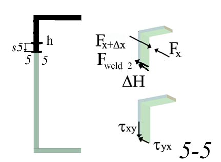
Figure 2.5.k
Theoretical rational:
(a) in the absence of the weld_1 and weld_2
![]()
![]()
![]() (area above the NA is
in compression).
(area above the NA is
in compression).
![]()
![]()
![]()
![]()
![]()
![]()
![]()
![]()
![]()
![]()
![]()
![]()
![]()
![]()
![]()
![]()
![]()
(f) the weld_1 effect and weld_2:
![]() the reaction induced
by the weld_1 on the cut cross-section is equal and has an opposite direction
the reaction induced
by the weld_1 on the cut cross-section is equal and has an opposite direction ![]()
![]()
![]()
![]()
![]()
![]() the reaction induced
by the weld_1 on the cut cross-section is equal and has an opposite direction
the reaction induced
by the weld_1 on the cut cross-section is equal and has an opposite direction ![]()
![]()
![]()
![]()
![]()
(g) the resultant shear stress on the cut cross-section is:
![]()
![]()
![]()
Numerical calculations:
![]()
![]()
![]() -
thickness of the cut at s2
-
thickness of the cut at s2
![]()
static moment about the neutral axis
 -
shear flow on the cut area if the weld wouldnt exist
-
shear flow on the cut area if the weld wouldnt exist
![]() -
shear flow on the cut area
-
shear flow on the cut area
 -
shear stress on the cut area
-
shear stress on the cut area
The variation of the shear stress is a second- order parabola. Only two values of the shear stress are necessary and they are calculated at the location at the lower weld on the vertical flange and at the junction between the vertical flange and the neutral axis location.
cut h
![]()
![]()
![]()
![]()
![]()
![]()
![]()
![]()
shear stress at the vertical flange at the lower weld position
cut i
![]()
![]()
![]()
![]()
![]()
![]()
![]()
![]()
![]()
![]()
shear stress at the neutral axis position
B.3.c.2.c Area A5
Theoretical rational:
![]()
![]()
![]() (area below the NA is
in tension).
(area below the NA is
in tension).
![]()
![]()
![]()
![]()
![]()
![]()
![]()
![]()
![]()
![]()
![]()
![]()
![]()
![]()
![]()
![]()
![]()
![]()
![]()
Numerical calculations:
![]()
![]()
![]() -
thickness of the cut at s3
-
thickness of the cut at s3

- static moment about the neutral axis
 -
shear flow on the cut area
-
shear flow on the cut area
 -
shear stress on the cut area
-
shear stress on the cut area
The variation of the shear stress is a second- order parabola. Only two values of the shear stress are necessary to be calculated and they are expressed at the location of the junction between the lower flange and the web and at the neutral axis location.
cut j
![]()
![]()
![]()
![]()
![]()
![]()
![]()
- shear stress at the junction between lower flange and web
cut i
![]()
![]()
![]()
![]()
![]()
![]()
![]()
![]()
![]()
- shear stress at the neutral axis
B.3.c.3 Lower
Flange (![]() shear stress)
shear stress)
The calculation
of the shear stress ![]() corresponding to the
lower flange is conducted in a similar manner with the calculation developed in
section B.3.c.1. The horizontal cut 6-6 is
made, as shown in Figure 2.5.l, at
distance s6 measured from l and increasing towards k.
corresponding to the
lower flange is conducted in a similar manner with the calculation developed in
section B.3.c.1. The horizontal cut 6-6 is
made, as shown in Figure 2.5.l, at
distance s6 measured from l and increasing towards k.
Figure 2.5.l
Theoretical rational:
![]()
![]()
![]() (area below the NA is
in tension)
(area below the NA is
in tension)
![]()
![]()
![]()
![]()
![]()
![]()
![]()
![]()
![]()
![]()
![]()
![]()
![]()
![]()
![]()
![]()
![]()
![]()
![]()
Numerical calculations:
![]()
![]()
![]() -
thickness of the cut at s3
-
thickness of the cut at s3
 -
static moment about the neutral axis
-
static moment about the neutral axis
 -
shear flow on the cut area
-
shear flow on the cut area
 -
shear stress on the cut area
-
shear stress on the cut area
The above
functions are particularized for the two limiting cuts of the segment kl. Only two values are sufficient because the
variation of the shear stress ![]() is linear.
is linear.
cut l
![]()
![]()
![]()
![]()
![]()
![]()
![]()
- shear stress at the face of the flange
cut k

![]()
![]()
![]()
![]()
![]()
![]()
![]()
![]()
- shear stress at the face of the web
? ? ? ? closed twin-wall cross-section??????
Problem 2.6
The longitudinal view and the cross-section of the structural steel bridge beam
are shown in Figure 2.6. The upper and lower bolts are of 10 mm and 12 mm diameter,
respectively. Calculate: (a) the geometrical characteristics of the
cross-section considering the existence of the bolts and without the bolts, (b)
the capable bending moment and shear force of the cross-section with and
without considering the bolt existence and
considering a material characterized by an allowable normal ![]() and shear
and shear ![]() stresses, (c) the
necessary spacing between the bolts (
stresses, (c) the
necessary spacing between the bolts (![]() and
and ![]() ) and (d) the effective thickness of the welds (
) and (d) the effective thickness of the welds (![]() ). For the calculations required at (d) and (e) consider a
shear force equal to half of the capable shear force of the cross-section.
). For the calculations required at (d) and (e) consider a
shear force equal to half of the capable shear force of the cross-section.
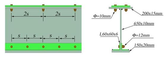
Figure 2.6
A. General Observations
A.1 The cross-section is subjected to non-uniform bending. Both Naviers and Jourawskis Formulas are applicable. The beam is made of steel and consequently, the allowable bending stress has an equal value for both tensile and compressive normal stress. Usually the existence of the bolts, which are reducing the effective area of the cross-section, is neglected when the cross-sectional geometrical properties are calculated. The error introduced by neglecting the bolt existence is negligible and is covered by the safety factor used in determining the allowable stresses of the material.
The calculation required at (a) evaluates the geometrical characteristics for both cases: a full cross-section and a reduced cross-section. A comparison is made. In engineering practice this dilemma is solved by placing the full-section in the cross-section of maximum moment. As it is concluded in a previous problem the shear force is primarily carried by the web, area little affected by the reduction.
A.2 Numerical Application
material data
![]() - allowable normal tensile and
compressive stress
- allowable normal tensile and
compressive stress
![]() - allowable shear stress
- allowable shear stress
cross-sectional dimensions
![]() - thickness of the first part of the
upper flange
- thickness of the first part of the
upper flange
![]() -width of the first part of the upper
flange
-width of the first part of the upper
flange
![]() - thickness of the second part of the
upper flange
- thickness of the second part of the
upper flange
![]() -width of the second part of the upper
flange
-width of the second part of the upper
flange
![]() - web thickness
- web thickness
![]() -
web height
-
web height
![]() - thickness of the first part of the
lower flange
- thickness of the first part of the
lower flange
![]() - web of the first part of the lower
flange
- web of the first part of the lower
flange
![]() - length of the angle
- length of the angle
![]() - thickness of the angle
- thickness of the angle
![]() - eccentricity of the angle
- eccentricity of the angle
![]() - area of the angle
- area of the angle
![]() - moment of inertia of the angle
- moment of inertia of the angle
bolts
![]() -
allowable shear stress
-
allowable shear stress
![]() -
allowable bearing stress
-
allowable bearing stress
![]() -
number of bolts used to connect the parts of the upper flange
-
number of bolts used to connect the parts of the upper flange
![]() - diameter of the upper bolts
- diameter of the upper bolts
![]()
![]()
![]() - length of the upper bolts
- length of the upper bolts
![]() -
number of bolts used to connect the parts of the lower flange
-
number of bolts used to connect the parts of the lower flange
![]() -
diameter of the lower bolts
-
diameter of the lower bolts
![]()
![]()
![]() -
length of the upper bolts
-
length of the upper bolts
![]() - position of the lower bolts
- position of the lower bolts
weld
![]() -
allowable shear stress
-
allowable shear stress
B. Calculations
B.1 Calculation of the Cross- Section Geometrical Characteristics
Note: the calculations are conducted using cm as unit.
B.1.a Full Cross-section (see Figure 2.6.a)
The area of the component parts and the total area of the cross-section, calculated under the assumption that the bolt holes are neglected, are:
![]()
![]()
![]()
- area of the first part of the upper flange
![]()
![]()
![]()
- area of the second part of the upper flange
![]()
![]()
![]() -
area of the web
-
area of the web
![]() -
area of the angle
-
area of the angle
![]()
![]()
![]() -
area of the first part of the lower flange
-
area of the first part of the lower flange
![]()
![]()
![]() -
total area
-
total area
The cross-section is symmetric against the vertical axis OYc and, consequently, only the vertical position of the centroid is necessary to be calculated. The coordinate system OYcZ coincides with the centroid of the web. The distances from the origin O to the centriods of the parts are:

![]()
![]()

![]()
![]()

![]()
![]()

![]()
![]()

![]()
![]() -
static moment
-
static moment

![]()
![]() -
centroid position
-
centroid position
The coordinate system is moved in the centroid C (the new coordinate system CYcZc) and the distances to the centroid of the parts are accordingly adjusted:
![]()
![]()
![]()
![]()
![]()
![]()
![]()
![]()
![]()
![]()
![]()
![]()
![]()
![]()
![]()
The centroidal moment of inertia about the axis CYcZc is obtained:


![]()
The section modulus considering the distances measured from the centroid to the extreme fibers of the cross-section:

![]()
![]()
![]()
![]()

![]()
![]()

![]()
![]()
![]()
![]()
![]()
B.1.b Effective Cross-section (see Figure 2.6.b)
The calculation is repeated considering the hole of the bolts. The position of the holes measured in the coordinate system OYcZ:


![]()

![]()
![]()
The corresponding hole areas are calculated as:
![]()
![]()
![]() - upper bolt
- upper bolt
![]()
![]()
![]() - lower bolt
- lower bolt
![]()
![]()
![]()
Note: A reduction area by 5% is calculated due the bolt existence.
The centroid of the effective area is obtained:
![]()
![]()
![]()

![]()
![]()
- position of the centroid of the effective cross-section
The new coordinate system CYcZ is located in the centroid of the effective cross-section. After correcting the centroidal distances measured from centroid of the effective cross-section to the centroid of the component areas, the centroidal moment of inertia of the effective cross-section against the axis CZc is obtained as:
![]()
![]()
![]()
![]()
![]()
![]()
![]()
![]()
![]()
![]()
![]()
![]()
![]()
![]()
![]()
![]()
![]()
![]()
![]()
![]()
![]()


![]()
Note: The ratio between the moments of inertia calculated is indicating a reduction with 6.5% when the bolts are considered. In engineering practice the bolts are not staggered all in the same cross-section.

The effective section modulus is calculated as:

![]()
![]()

![]()
![]()

![]()
![]()

![]()
![]()
![]()
![]()
![]()
B.2 Calculation of Bending Capacity of the Cross-Section
B.2.a Full Cross-section
The capable bending moment of the full cross-section is obtained as:
![]()
![]()
![]()
B.2.b Effective Cross-section
The capable bending moment of the effective cross-section is calculated in a similar manner:
![]()
![]()
![]()
The ratio of the capable bending moment is:

Note: As expected, a reduction in the bending capacity of the effective cross-section is emphasized. This reduction represents a small percentage of the bending capacity when the bolts existence is neglected. For this reason and some other consideration related to the safety factor used in the calculation of the allowable normal stress in the engineering practice the bolts are not considered and the moment of inertia of the full cross-section is usually used.
B.3 Calculation of Shear Capacity of the Cross-Section
B.3.a Full Cross-section
Using the Jourawskis Formula the capable shear force is calculated:

![]()
![]()
where the maximum static moment about the neutral axis is obtained as:

![]()
![]()
B.3.b Effective Cross-section
The calculation og the capable shear force of the cross-section is conducted:

![]()
![]()


![]()
The ratio of the capable shear forces calculated considering the full section and the section with bolts is:

Note: The reduction induced by the bolts existence is insignificant and shows that the bolts can be excluded from the calculation involving the shear force.
B.4 Calculation of the Bolts Spacing
The calculation requires a shear force ![]() :
:
![]()
![]()
![]()
B.4.a Upper Bolts
The shear flow corresponding to the upper bolts is calculated as:

![]()
![]()
where the static moment is:
![]()
![]()
![]()
The 10 mm bolt capacity is obtained calculating the minimum between the bolt capacities in bearing and shearing:
![]() - number of shearing sections of the
bolt
- number of shearing sections of the
bolt

![]()
![]()
![]()
![]()
![]()
![]()
![]()
![]()
The spacing of the upper bolts is obtained:

![]()
![]()
B.4.b Lower Bolts
The shear flow corresponding to the upper bolts is calculated as:

![]()
![]()
where the static moment is:
![]()
![]()
![]()
The 12 mm bolt capacity is obtained calculating the minimum between the bolt capacities in bearing and shearing:
![]() -
number of shearing sections of the bolt
-
number of shearing sections of the bolt

![]()
![]()
![]()
![]()
![]()
![]()
![]()
![]()
The spacing of the lower bolts is obtained:

![]()
![]()
The lower and upper bolts are both placed in the same cross-section as required by the text. Then, the spacing is calculated as:
![]()
![]()
![]()
A rounded value is chosen to match the spacing:
![]()
The verification of the bolts is conducted for the new spacing for exercising purposes only:
![]()
![]()
B.5 Sizing of the Welds
B.5.a Upper Welds
The shear flow in the upper welds is calculated:

![]()
![]()
where the corresponding static moment is obtained:
![]()
![]()
![]()
The upper welds capacity is calculated:
![]()
![]()
The effective thickness of the upper welds is obtained from the equation:
![]()
and consequently,

![]()
![]()
B.5.b Lower Welds
The shear flow in the lower welds is calculated:

![]()
![]()
where the corresponding static moment is obtained:
![]()
![]()
![]()
The lower welds capacity is calculated:
![]()
![]()
The effective thickness of the lower welds is obtained from the equation:
![]()

![]()
![]()
Problem 2.7
Considering the steel beam shown in Figure 2.7 conduct the following tasks: (a)
calculate and draw the pertinent cross-sectional resultant diagrams, (b)
calculate the cross-section geometrical characteristics, (c) verify the beam
for strength employing the following allowable normal ![]() and shear
and shear ![]() stresses, (d) size the
welds (the effective throat) using the allowable shear stress
stresses, (d) size the
welds (the effective throat) using the allowable shear stress ![]() , and (e) calculate and draw the normal and shear stresses in
cross-section S located at 1m right of end
point of the uniform distributed load.
, and (e) calculate and draw the normal and shear stresses in
cross-section S located at 1m right of end
point of the uniform distributed load.
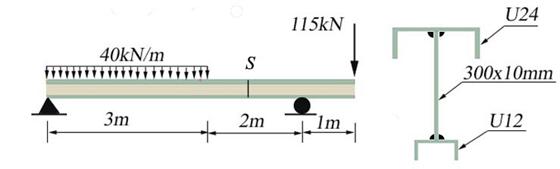
Figure 2.7
A. General Observations
A.1 The loads are acting in the vertical plane and, consequently, the steel beam is subjected to non-uniform bending. Both Naviers and Jourawskis Formulas are applicable. The beam is made of steel and consequently, the allowable bending stress has an equal value for both tensile and compressive normal stress.
A.2 Numerical Application
loading and dimensions
![]()
![]()
![]()
![]()
![]()
material data
![]() - allowable normal tensile and
compressive stress
- allowable normal tensile and
compressive stress
![]()
![]()
![]() - allowable shear stress
- allowable shear stress
cross-sectional dimensions
- Shape 1: Rectangular Web (300x10 mm)
![]() - height
- height
![]() - thickness
- thickness
- Shape 2: U24
![]() - height of the shape
- height of the shape
![]() - thickness of the web
- thickness of the web
![]() - length of the flange
- length of the flange
![]() - thickness of the flange
- thickness of the flange
![]() - eccentricity
- eccentricity
![]() - area
- area
![]() - moment of inertia about an axis parallel
to z axis
- moment of inertia about an axis parallel
to z axis
- Shape 3: U12
![]() - height of the shape
- height of the shape
![]() - thickness of the web
- thickness of the web
![]() - length of the flange
- length of the flange
![]() - thickness of the flange
- thickness of the flange
![]() - eccentricity
- eccentricity
![]() - area
- area
![]() - moment of inertia about an axis
parallel to z axis
- moment of inertia about an axis
parallel to z axis
welds
![]() - number of superior welds
- number of superior welds
![]() - number of inferior welds
- number of inferior welds
![]()
![]()
![]()
- allowable shear stress
B. Calculations
B.1 Cross-Sectional Internal Resultants (see Figure 2.a)
Note: The cross-sectional internal resultants are calculated and graphically represented as detailed explained in Chapter 3 of volume I.
B.1.a Calculation of the Reaction Forces
The support restrictions are replaced by the corresponding reaction forces. The reaction forces together with the loads represent the free-body diagram of the beam. Due to the fact that the loads and reaction forces are located in the vertical plane OXY only three (3) global equilibrium equations are written for the entire free-body diagram of the beam. They are:
 - projection of the forces on the
horizontal direction OX
- projection of the forces on the
horizontal direction OX
 - sum of moments about direction OZ in point 1
 - sum of moments about direction OZ in point 3
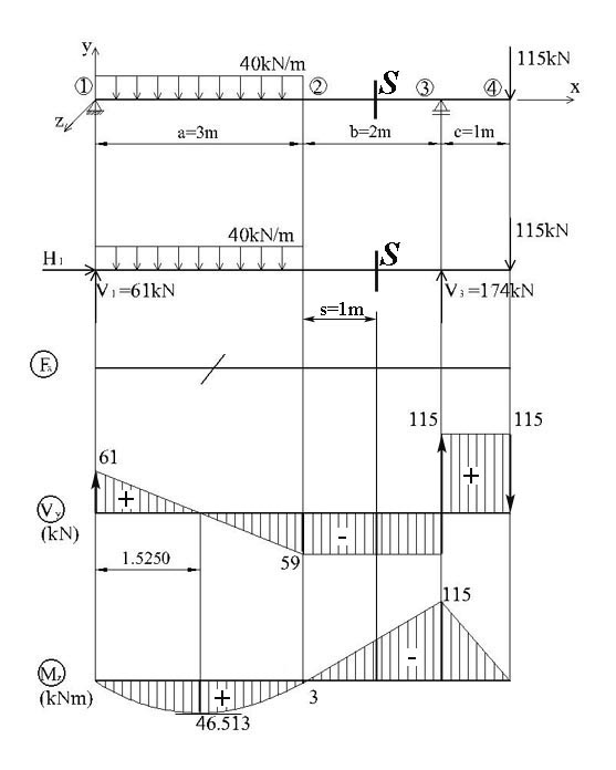
Figure 2.a
Explicitly, the above equations are written as:
![]()
![]()
![]()
To verify the calculations
conducted above the projection equation  on the OY axis is employed:
![]()
![]() verify
verify
B.1.a Calculation of the Shear Force Vy
The value of the shear force at the locations indicated on Figure 2.a are obtained as:
![]()
![]()
![]()
![]()
![]()
![]()
![]()
![]()
![]()
![]()
![]()
![]()
![]()
![]()
![]()
![]()
![]()
![]()
![]()
![]()
![]()
The shear force in the interval 12 changes the sign from positive to negative, and consequently, a value of zero appears in a cross-section located at distance x from point 1. The expression of the shear force on the interval 12 is:
![]()
The distance x is calculated:

![]()
![]()
B.1.b Calculation of the Bending Moment Mz
The value of the bending moment at the locations indicated on Figure 2.a are obtained as:
![]()
![]()
![]()
![]()
![]()
![]()
![]()
![]()
![]()
![]()
![]()
![]()
![]()
B.2 Calculation of the Cross- Section Geometrical Characteristics (see Figure 2.b)
Note: the calculations are conducted using cm as unit.
The cross-section is composed from three shapes: a rectangular shape 300x10mm, U24 and U12. The area of the cross-section is calculated:
![]()
![]()
![]()
The original coordinate system is attached to point C1, the centroid of the rectangular shape. The distances from the origin of the coordinate system to the centroid of each individual shape are:
![]()

![]()
![]()

![]()
![]()
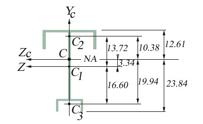
Figure 2.b
The position of the centroid is obtained:

![]()
![]()
![]() (due to the cross-section symmetry)
(due to the cross-section symmetry)
A new coordinate system, attached to the cross-section centroid C, is now employed. The new positions of the centroids of each individual shape are established as:
![]()
![]()
![]()
![]()
![]()
![]()
![]()
![]()
![]()
The only moment of inertia necessary to be calculated is:


![]()
The distances to the extreme fibers of the cross-section are:
![]()
![]()
![]()
![]()
![]()
![]()
The sectional modulus is calculated:

![]()
![]()

![]()
![]()
![]()
![]()
![]()
B.3 Verification of the Cross-Section for Strength
B.3.a Normal Stress Verification (sx Verification)
The verification of the normal stress is conducted in the cross-section where the maximum absolute bending moment is reached. This cross-section is identified by surveying the bending moment diagram shown in Figure 2.a.
![]()
where:
![]()
![]()
![]()

![]()
![]()

![]()
![]()
![]()
![]()
![]()
The normal stress diagram in the cross-section corresponding to the maximum bending moment is shown in Figure 2.7c.
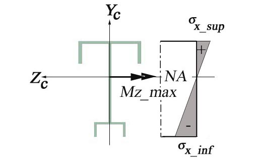
Figure 2.7c
An alternative approach, using the sectional modulus, is the following:


where:
![]()
![]()
![]()


![]()
![]()
B.3.b Shear Stress Verification (txy Verification)
The shear stress verification is conducted in the cross-section where the shear force reaches the maximum absolute. This cross-section is identified by surveying the shear force diagram shown in Figure 2.a. The formula used in the shear stress verification is:

where:
![]()
![]()
![]()

![]()
![]()
the static moment of the area located above the neutral axis (NA).

![]()
![]()
![]()
B.4 Sizing of the Welds
B.4.a The Upper Welds
The sizing of the upper welds is performed using the following formula:
![]()
The shear capacity of the upper welds is calculated as:
![]()
The shear flow in the upper welds is calculated:

![]()
![]()
where:
![]()
![]()
![]()
- the static moment of the U24 about the neutral axis (NA)
The effective throat of the upper weld is the only unknown quantity and is calculated as:

![]()
![]()
B.4.bThe Lower Welds
The sizing of the lower welds is performed using the following formula:
![]()
The shear capacity of the lower welds is calculated as:
![]()
The shear flow in the lower welds is calculated:

![]()
![]()
where:
![]()
![]()
![]()
The effective throat of the lower weld is the only unknown quantity and is calculated as:

![]()
![]()
B.5 Stress Diagrams in Section S.
The bending moment and the shear force in the cross-section S are:
![]()
![]()
![]()
![]()
![]()
![]()
![]()
B.5.a Normal Stress Diagram (sx Diagram see Figure 2.d)
The normal stress (sx) diagram in the cross-section S is constructed in a similar manner with the sx diagram used in the calculation of the sx_max. The variation of the normal stress on the cross-section is linear in accordance to the Naviers Formula and only the values at the extreme fibers a necessary to be calculated.

Figure 2.d

![]()
![]()

![]()
![]()
B.5.b
The shear flow and stress diagram is calculated following the explanations regarding the application of the Jurawskis Formula detailed in the theoretical paragraph of the chapter.
The cross-section is divided into six distinct rectangular areas, A1 through A6, where the Jurawskis formula is applicable. This division is shown in Figure 2.e. Each area is delineated by two cuts (A1:a-b or a-b, A2:c-d or c-d, A3:e-f, A4:g-f, A5:k-j or k-j, A6:i-g or i-h). The variation of the corresponding shear stress is calculated on each of the six areas.
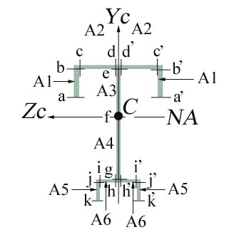
Figure 2.e
Note: An infinitesimal element of the beam starting from the cross-section S and having a length Dx is isolated from the entire beam.
For each cut the
corresponding free body diagram is drawn. The resulting forces ![]() and
and ![]() on each face of the resulting free body are indicated
function of the signs of the bending moment and shear force acting in the
cross-section S. For the equilibrium
to be realized
on each face of the resulting free body are indicated
function of the signs of the bending moment and shear force acting in the
cross-section S. For the equilibrium
to be realized
B.5.b.1 Calculation of the Shear Stress on Area A1 (see Figure 2.f)
The horizontal cut 1-1 is made at distance s1 measured from a and increasing towards b.
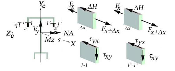
Figure 2.f
Theoretical rational:
![]()
![]()
![]() (area above the NA is
in tension).
(area above the NA is
in tension).
![]()
![]()
![]()
![]()
![]()
![]()
![]()
![]()
![]()
![]()
![]()
![]()
![]()
![]()
![]()
![]()
![]()
![]()
![]()
Numerical calculations:
![]()
![]()
 - thickness of the cut at s1
![]()
- static moment about the neutral axis
 - shear flow on the cut area
 -
shear stress on the cut area
-
shear stress on the cut area
The above functions are particularized for the two limiting cuts of the segment ab.
cut a
![]()
![]()
![]()
![]()
![]()
![]()
![]()
cut b
![]()
![]()
![]()
![]()
![]()
![]()
![]()
![]()
![]()
The calculation for the segment ab is conducted in a similar manner as for the segment ab and the shear stress is symmetric.
B.5.b.2 Calculation of the Shear Stress on Area A2 (see Figure 2.g)
The vertical cut 2-2 is made at distance s2 measured from c and increasing towards d.
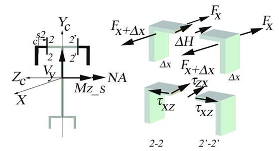
Figure 2.g
Theoretical rational:
![]()
![]()
![]() (area above the NA is
in tension).
(area above the NA is
in tension).
![]()
![]()
![]()
![]()
![]()
![]()
![]()
![]()
![]()
![]()
![]()
![]()
![]()
![]()
![]()
![]()
![]()
![]()
![]()
Numerical calculations:
![]()
![]()
![]() -
thickness of the cut at s2
-
thickness of the cut at s2

- static moment about the neutral axis
 -
shear flow on the cut area
-
shear flow on the cut area
 -
shear stress on the cut area
-
shear stress on the cut area
The above functions are particularized for the two limiting cuts of the segment cd:
cut c
![]()
![]()
![]()
![]()
![]()
![]()
![]()
cut d

![]()
![]()
![]()
![]()
![]()
![]()
![]()
![]()
The calculation for the segment cd is conducted in a similar manner as for the segment cd and the shear stress is symmetric.
B.5.b.3 Calculation of the Shear Stress on Area A3 (see Figure 2.h)
The horizontal cut 3-3 is made at distance s3 measured from e and increasing towards f.
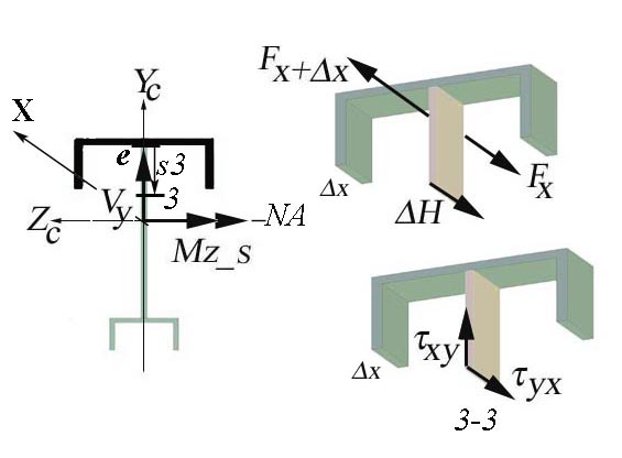
Figure 2.h
Theoretical rational:
![]()
![]()
![]() (area above the NA is
in tension).
(area above the NA is
in tension).
![]()
![]()
![]()
![]()
![]()
![]()
![]()
![]()
![]()
![]()
![]()
![]()
![]()
![]()
![]()
![]()
![]()
![]()
![]()
Numerical calculations:
![]()
![]()
![]() -
thickness of the cut at s3
-
thickness of the cut at s3
![]()
- static moment about the neutral axis
 -
shear flow on the cut area
-
shear flow on the cut area
 -
shear stress on the cut area
-
shear stress on the cut area
The above functions are particularized for the two limiting cuts of the segment ef:.
cut e
![]()
![]()
![]()
![]()
![]()
![]()
![]()
cut f
![]()
![]()
![]()
![]()
![]()
![]()
![]()
![]()
![]()
B.5.b.4 Calculation of the Shear Stress on Area A5 (see Figure 2.i)
The horizontal cut 5-5 is made at distance s5 measured from k and increasing towards j.
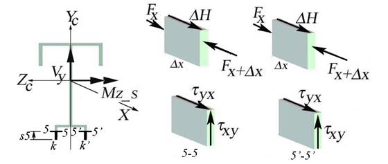
Figure 2.i
Theoretical rational:
![]()
![]()
![]() (area below the NA is
in compression).
(area below the NA is
in compression).
![]()
![]()
![]()
![]()
![]()
![]()
![]()
![]()
![]()
![]()
![]()
![]()
![]()
![]()
![]()
![]()
![]()
![]()
![]()
Numerical calculations:
![]()
![]()
![]() -
thickness of the cut at s5
-
thickness of the cut at s5
![]() -
static moment about the neutral axis
-
static moment about the neutral axis
 -
shear flow on the cut area
-
shear flow on the cut area
 -
shear stress on the cut area
-
shear stress on the cut area
The above functions are particularized for the two limiting cuts of the segment kj:.
cut k
![]()
![]()
![]()
![]()
![]()
![]()
![]()
cut j
![]()
![]()
![]() -
thickness of the cut at s5
-
thickness of the cut at s5
![]()
![]()
![]()
![]()
![]()
![]()
The calculation for the segment kj is conducted in a similar manner as for the segment kj and the shear stress is symmetric.
B.5.b.5 Calculation of the Shear Stress on Area A6 (see Figure 2.j)
The vertical cut 6-6 is made at distance s6 measured from i and increasing towards h.
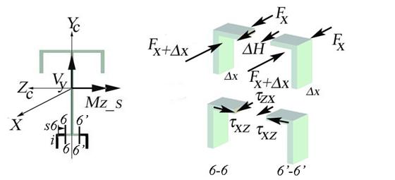
Figure 2.j
Theoretical rational:
![]()
![]()
![]() (area below the NA is
in compression).
(area below the NA is
in compression).
![]()
![]()
![]()
![]()
![]()
![]()
![]()
![]()
![]()
![]()
![]()
![]()
![]()
![]()
![]()
![]()
![]()
![]()
![]()
Numerical calculations:
![]()
![]()
![]() -
thickness of the cut at s6
-
thickness of the cut at s6

- static moment about the neutral axis
 -
shear flow on the cut area
-
shear flow on the cut area
 -
shear stress on the cut area
-
shear stress on the cut area
The above functions are particularized for the two limiting cuts of the segment kj:.
cut i
![]()
![]()
![]()
![]()
![]()
![]()
![]()
cut j

![]()
![]()
![]()
![]()
![]()
![]()
![]()
![]()
The calculation for the segment ij is conducted in a similar manner as for the segment ij and the shear stress is symmetric.
B.5.b.6 Calculation of the Shear Stress on Area A4 (see Figure 2.k)
The horizontal cut 4-4 is made at distance s3 measured from g and increasing towards f.
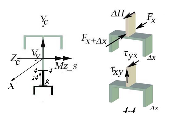
Figure 2.k
Theoretical rational:
![]()
![]()
![]() (area below the NA is
in compression).
(area below the NA is
in compression).
![]()
![]()
![]()
![]()
![]()
![]()
![]()
![]()
![]()
![]()
![]()
![]()
![]()
![]()
![]()
![]()
![]()
![]()
![]()
Numerical calculations:
![]()
![]()
![]() -
thickness of the cut at s4
-
thickness of the cut at s4
![]()
static moment about the neutral axis
 -
shear flow on the cut area
-
shear flow on the cut area
 -
shear stress on the cut area
-
shear stress on the cut area
cut g
![]()
![]()
![]()
![]()
![]()
![]()
![]()
cut f
![]()
![]()
![]()
![]()
![]()
![]()
![]()
![]()
![]()
3 Proposed Problems
Problem 3.1 The cross-section of the structural steel wide-flange beam I40, shown in Figure 3.1, is subjected to pure bending. Alternatively considering the situations pictured in Figures 3.1.a and 3.1.b and assuming that the allowable bending stress is sallow = 200 MPa, calculate: (a) the flexural stress and strain distribution on the cross-section and (b) the maximum bending moment which can be applied.
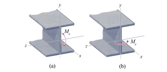
Figure 3.1
Problems 3.2 The cross-section shown in Figure 3.2 is subjected to pure bending.
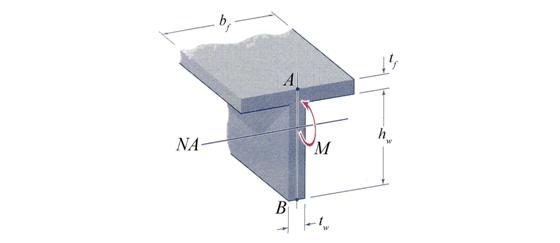
Figure 3.2
Conduct the
following tasks: (a) Draw the flexural stress and strain distributions
considering the following dimensions: bf = 20 cm, t f = 5
cm, hw =15 cm, and tw = 2 cm, (b) Calculate the capable
bending moment of the cross-section is the allowable tensile and compressive
normal stress is sallow =
220 MPa, and (c) Determine the stresses at points A and B if a bending
moment ![]() is acting on the
cross-section.
is acting on the
cross-section.
Problems 3.3 A wood beam made from three boards that are glued together to form a single beam, as shown in Figure 3.3, is subjected to pure bending. Obtain an analytical expression for: (a) the tensile and compression maximum stresses and draw the stress distribution on the cross-section, (b) the total force acting on the top board and (c) for a=10 cm calculate the capable bending moment if the allowable tensile and compressive stresses are sall_tens =35 MPa and sall_compr =25 MPa, respectively.
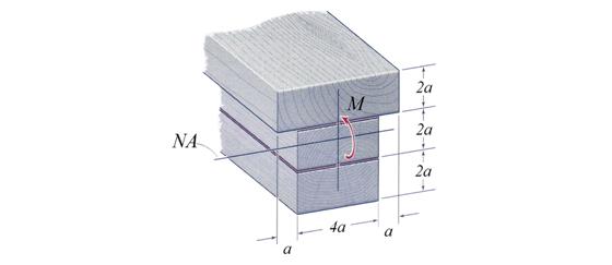
Figure 3.3
Problems 3.4 A tee-beam shaped cross-section beam, with dimensions shown in Figure 3.4, is subjected to a bending moment of magnitude of M=40 kN. Draw the flexural stress and strain distributions and calculate the maximum tensile and flexural stress at this cross-section.
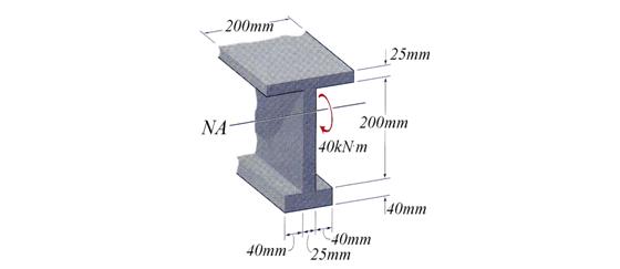
Figure 3.4
Problem 3.5 If the allowable shear stress (for shear parallel to the grain of the wood) in a timber beam cross-section b=10 cm and h=15 cm, shown in Figure 3.5, is tall = 20 MPa, draw the shear stress diagram and calculate the maximum transversal shear force, V, which can be sustained by the wood beam.
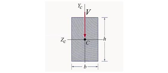
Figure 3.5
Problem 3.6 Using Jurawskis Formula, determine an expression for the shear stress at the neutral-axis of the circular and tubular cross-sections shown in Figures 3.6. Conduct a numerical application for the following data: d=10 cm and di=5 cm.
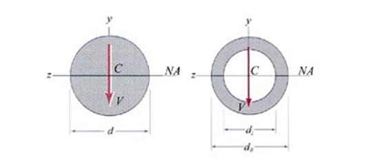
Figure 3.6
Problem 6.3.7 A vertical shear force V = 200 kN is applied to the cross-section shown in Figure 6.3.3 Considering the following dimensions: h = 320 mm, hw = 300 mm, b = 160mm and tw = 8mm, calculate: (a) the distribution of the shear stress on the cross-section and (b) the shear force carried by the web.
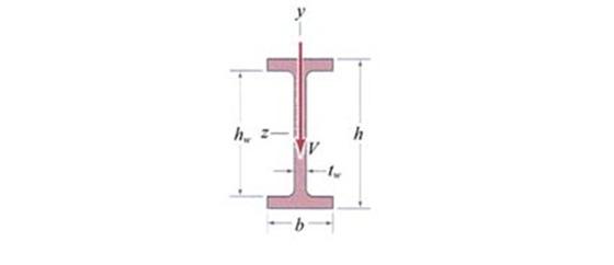
Figure 3.7
Problem 3.8
Two wide-flange beams I20 and I40, respectively, are subjected to the
same magnitude vertical shear force, V.
Determine: (a) the distribution of the shear stresses for each cross-section,
(b) the maximum shear force allowed by each wide-flange beam if the allowable
shear stress is ![]() , (c) the shear force carried by the webs of each beam and
(c) the ration of the maximum shear stresses.
, (c) the shear force carried by the webs of each beam and
(c) the ration of the maximum shear stresses.
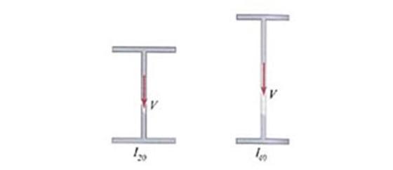
Figure 3.8
Problem 3.9 Repeat the calculations required in problem 3.8 for the cross-sections shown in Figure 3.9. Consider as numerical application t=1.5 cm.
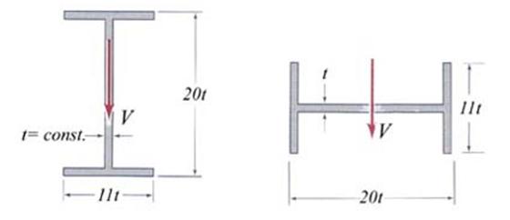
Figure 3.9
Problem 3.10 The tee cross-section shown in Figure 3.10. is subjected to a vertical shear force V. Calculate: (a) the expression of the shear stress distribution and (b) the vertical shear force in the web. Consider a numerical application for t=1 cm.
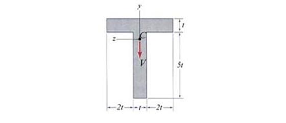
Figure 3.10
Problem 3.11 Repeat the calculations required by problem 6.3.10 using the dimensions shown in Figure 3.11.
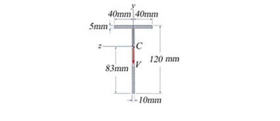
Figure 3.11
Problem 3.12 The channel cross-section shown in Figure 3.12 is subjected to a vertical force V = 10 kN. Calculate: (a) the shear stress distribution, (b) the shear stress at point A and B and (c) the vertical shear forces carried by the flanges.
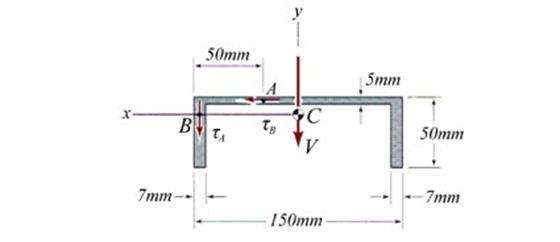
Figure 3.12
Problem 3.13 Considering the thin-wall closed cross-section shown in Figure 3.13 subjected to a vertical shear force V, calculate: (a) the shear stress distribution and (b) the vertical shear force in the webs.
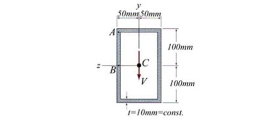
Figure 3.13
Problem 3.14 The tubular thin-wall closed cross-sections shown in Figure 3.14 are subjected to a vertical cross-section V. Calculate: (a) the shear stress distribution in the cross-sections, (b) the ratio of the maximum shear stresses and (c) the ratio of the shear force in the webs. Consider a numerical application for t=10 mm.
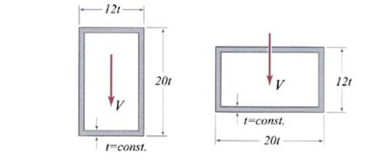
Figure 3.14
Problem 3.15 Repeat the requirements of problem 3.14 considering the cross-section shown in Figure 3.15.

Figure 3.15
Problem 3.16
The steel plate girder pictured in Figure 3.16 is fabricated by welding
together two horizontal plates to a vertical steel plate. Using the dimensions
shown in the figure and considering for the material an allowable shear stress of
![]() , (a) calculate the allowable shear force V in the cross-section and (b) size the
welds considering an allowable shear stress of
, (a) calculate the allowable shear force V in the cross-section and (b) size the
welds considering an allowable shear stress of ![]() .
.
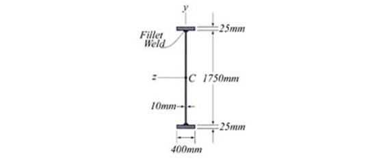
Figure 3.16
Problem 3.17 The I36
steel wide-flange beam, shown in Figure 3.17, is strengthened by welding on its
flanges two additional 175 mm x 10 mm
steel plates. Considering that a vertical shear force V is acting in the cross-section centroid calculate: (a) the shear stress
distribution in the original and strengthen cross-sections, (b) the allowable vertical
shear forces if the material is characterized by an allowable shear stress ![]() , and (c) size the weds considering that the weld shear
stress is
, and (c) size the weds considering that the weld shear
stress is ![]() .
.
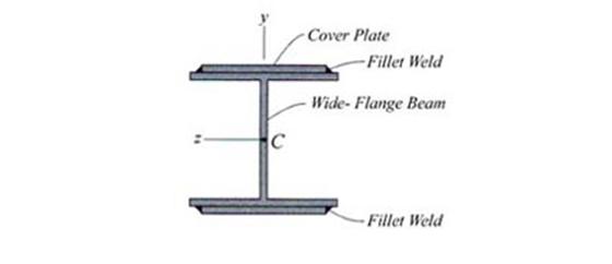
Figure 3.17
Problem 3.18
The tee steel beam shown in Figure 3.18 is fabricated by welding together two
steel plates and is subjected by a vertical shear force V. Calculate: (a) the distribution of the shear stress in the
cross-section and (b) the allowable shear force if the weld has a effective
thickness ![]() and
and ![]() .
.
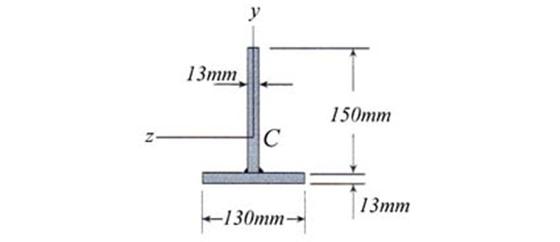
Figure 3.18
Problem 3.19 An I26 steel wide-flange beam subjected to a vertical shear force V is strengthened by bolting two additional U14 steel channels.
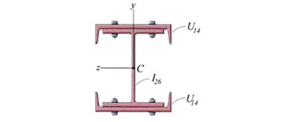
Figure 3.19
The strengthen
cross-section is shown in Figure 3.19. Calculate: (a) the shear stress
distribution in the web of the original and strengthen cross-sections and (b)
the maximum allowable vertical shear force in the strengthen cross-section if
the bolts have a diameter ![]() , are longitudinally spaced at
, are longitudinally spaced at ![]() and are made of a
material with allowable bearing and shear stresses of
and are made of a
material with allowable bearing and shear stresses of ![]() and
and ![]() .
.
Problem 3.20
A steel beam is built up from a I40 wide-flange beam and two 155mm x 152 mm cover plates as shown in Figure 3.20. Calculate the
allowable shear force and bending moment in the original and strengthened
cross-sections considering a material characterized by ![]() , and
, and ![]() . If the bolts are
. If the bolts are ![]() and are made of a
material with allowable bearing and shear stresses of
and are made of a
material with allowable bearing and shear stresses of ![]() and
and ![]() find the required
spacing.
find the required
spacing.
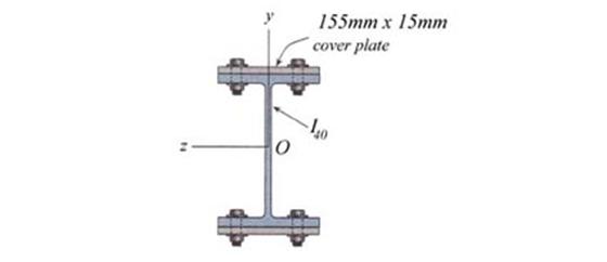
Figure 3.20
Problem 3.21 Two wood box beams, shown in Figure 3.21, have identical cross-sections. Considering a vertical shear force V = 5 kN and a bending moment M=50 KN*m calculate: (a) the normal and shear stress distributions in the cross-section, (b) the maximum spacing between the nails for each nail arrangement considering that the nail has an allowable shear force of 250 kN and are longitudinally spaced at 50 mm.
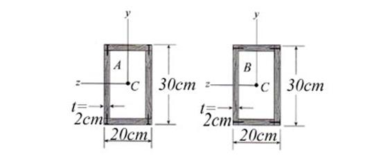
Figure 3.21
Problems 3.22
and 3.23 For the wood beams shown in Figures 3.22 and 3.23 calculate: (a)
the internal resultants diagrams and draw their plots, (b) the distributions of
the normal tensile and compressive stresses corresponding to the cross-section
where maximum stresses appear, (c) calculate the distribution of the shear
stress in the cross-section where maximum shear stress appears, (d) verify the
beam using the following allowable stresses ![]() ,
,![]() , and
, and ![]() .
.
.
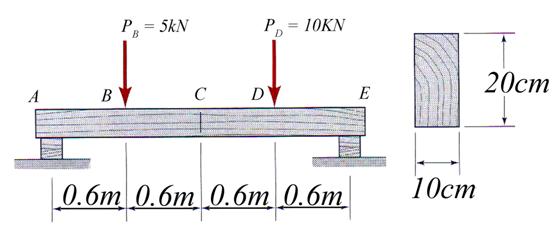
Figure 3.22
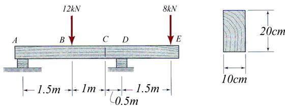
Figure 3.23
Problem 3.24 The timber beam shown in Figure 3.24 with 200 mm x 300 mm rectangular
cross-section is subjected to the following vertical concentrated loads: Pg = 15 kN and Pc = 25 kN. Calculate: (a)
the distribution of the flexural stress in the cross-section where maximum
appears, (b) the distribution of the shear stress on the cross where maximum appears
and (c) verify the beam considering the following allowable stresses: ![]() ,
,![]() , and
, and ![]() .
.
.
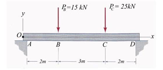
Figure 3.24
Problem 3.25 The
beam shown in Figure 3.25 is made of timber with the following allowable
stresses:![]() ,
,![]() , and
, and ![]() . Calculate: (a) the distribution of the flexural stress in
the cross-section where maximum appears, (b) the distribution of the shear
stress on the cross where maximum appears and (c) verify the beam and (d) find
the necessary spacing between the nails if nails
. Calculate: (a) the distribution of the flexural stress in
the cross-section where maximum appears, (b) the distribution of the shear
stress on the cross where maximum appears and (c) verify the beam and (d) find
the necessary spacing between the nails if nails ![]() and
and  are employed to
realize the connection.
are employed to
realize the connection.
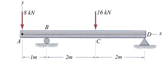
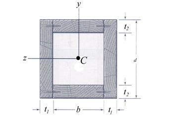
Figure 3.25
Problems 3.26
through 3.31 For the steel beams shown in Figures 3.26 and 3.31 calculate:
(a) the internal resultants diagrams and draw their plots, (b) the
distributions of the normal tensile and compressive stresses corresponding to
the cross-section where maximum stresses appear, (c) calculate the distribution
of the shear stress in the cross-section where maximum shear stress appears,
(d) verify the beam using the following allowable stresses ![]() and
and  , and (d) assuming an welded connection between the web and
flanges with
, and (d) assuming an welded connection between the web and
flanges with ![]() size the welds .
size the welds .
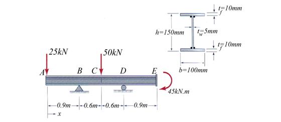
Figure 3.26
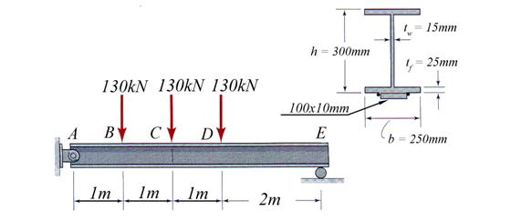
Figure 3.27
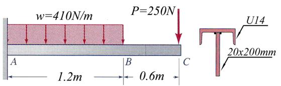
Figure 3.28
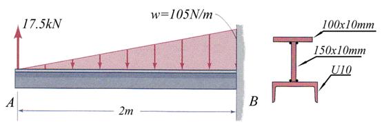
Figure 3.29
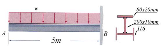 Figure 3.30
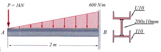
Figure 3.31
Problem 3.32
and 3.33 The beams shown in Figures 3.32 and 3.33 are made of I32 structural steel. Calculate: (a) the
internal resultants diagrams and plot the diagrams, (b) the flexural stress and
shear stress distributions in the cross-section right of B, (c) identify the cross-sections where the maximum normal and
shear stresses are and draw the corresponding distributions (d) verify the beam
considering the following allowable stresses ![]() and , (d) the vertical shear force in the web.
and , (d) the vertical shear force in the web.
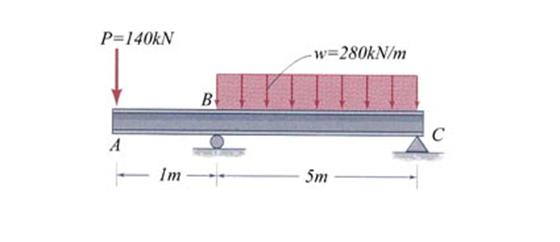
Figure 3.32
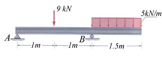
Figure 3.33
Problems 3.34
through 6.3.37 The beams shown in Figures 3.34 through 6.3.37 have the
cross-section made of I shape type
laminated steel. Determine the profile required if it is assumed that the
allowable tensile and compressive stresses are both equal to ![]() and .Draw the normal
and shear stresses diagrams in cross-section C.
and .Draw the normal
and shear stresses diagrams in cross-section C.
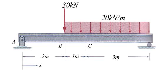
Figure 3.34
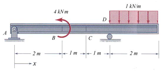
Figure 3.35
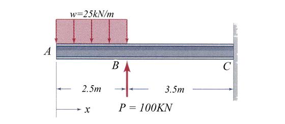
Figure 3.37
Problem 3.38
The beam illustrated in Figure 3.38 is made of wood which allows equal flexural
tensile and compressive stresses ![]() and
and ![]() . Calculate the
required dimensions for the cross-section, assuming the ratio height to width is 1.5. Draw the corresponding normal stress and shear stress diagrams
for the cross-section located at right of point C.
. Calculate the
required dimensions for the cross-section, assuming the ratio height to width is 1.5. Draw the corresponding normal stress and shear stress diagrams
for the cross-section located at right of point C.
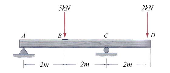
Figure 3.38
Problem 3.39
The laminated beam shown in Figure 3.39 is made by gluing together n planks of width b and thickness t. Derive
a formula for h=n*t and b considering that the wood has the
following allowable stresses: ![]() ,
, ![]() and
and ![]() . Assume that the
thickness of each glue layer is negligible and that the laminated beam behaves
like an ordinary wood beam. Calculate the number of required for the lightest
timber beam if the fallowing data is considered: b = 200 mm, L= 5 m, P = 9 kN and t = 50 mm.
. Assume that the
thickness of each glue layer is negligible and that the laminated beam behaves
like an ordinary wood beam. Calculate the number of required for the lightest
timber beam if the fallowing data is considered: b = 200 mm, L= 5 m, P = 9 kN and t = 50 mm.
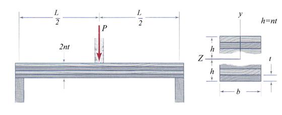
Figure 3.39
Problem 3.40
Locate the roller support B of the
beam shown in Figure 3.40 such that the beam AD has an equal magnitude of the maximum positive and negative
moments. Assuming PA = 30 kN,
PC = 40 kN, L = 1.5 m and an equal flexural tensile and compressive stresses ![]() for the steel, determine the required I shape.
for the steel, determine the required I shape.
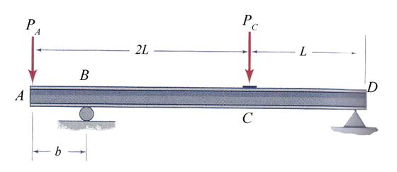
Figure 3.40
Problem 3.41 An electrical
switch is fabricated as shown in Figure 3.41. In the on position the button D moves down and applies a vertical
force P=50kN on the tip C of the copper plate AC. Assuming that the plate AC has a
rectangular cross-section and the copper is characterized by the following
allowable stresses ![]() and
and ![]() , calculate the required dimensions of the cross-section.
, calculate the required dimensions of the cross-section.
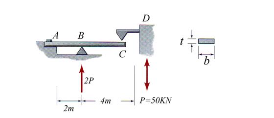
Figure 3.41
Problem 3.42
and 3.43 The beam illustrated in Figures 3.42 and 3.42 are made of wood
which allows equal flexural tensile and compressive stresses ![]() and
and ![]() . Calculate the
required dimensions for the rectangular cross-section, assuming the ratio height to width is 1.5.
. Calculate the
required dimensions for the rectangular cross-section, assuming the ratio height to width is 1.5.
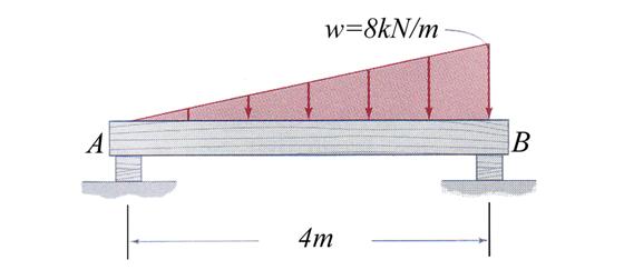
Figure 3.42
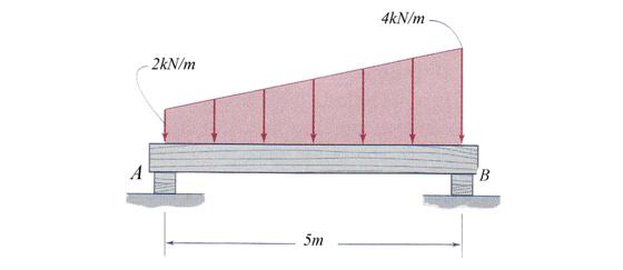
Figure 3.43
Problem 3.44
through 3.46 The steel beams shown in Figures 3.45 through 3.46 are
assembled from same type structural shapes. Determine the of size necessary
structural shapes, considering the following allowable stresses for the steel: ![]() and . Calculate the spacing between the bolts assuming a bolt diameter
and . Calculate the spacing between the bolts assuming a bolt diameter
![]() . The allowable stresses in the bolts are:
. The allowable stresses in the bolts are: ![]() and
and ![]()
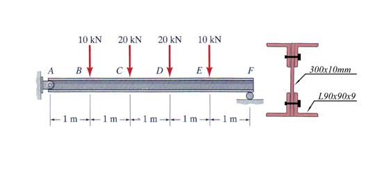
Figure 3.44
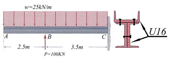
Figure 3.45
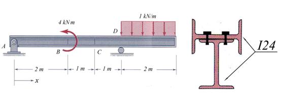
Figure 3.46
Problem 3.47
and 3.48 The beam shown in Figures 3.47 and 3.48 are made of structural
steel characterized by ![]() and allowable stresses. Calculate:
(a) the internal resultants diagrams, (b) the geometrical characteristics of
the cross-section, (c) the flexural and shear stress distribution in the
cross-sections where maximum values are obtained, (d) the maximum distributed
force w carried by the beam, (e) the vertical shear force in the web and (f)
the effective thickness of the weld considering
and allowable stresses. Calculate:
(a) the internal resultants diagrams, (b) the geometrical characteristics of
the cross-section, (c) the flexural and shear stress distribution in the
cross-sections where maximum values are obtained, (d) the maximum distributed
force w carried by the beam, (e) the vertical shear force in the web and (f)
the effective thickness of the weld considering ![]() .
.
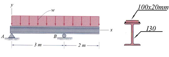
Figure 3.47
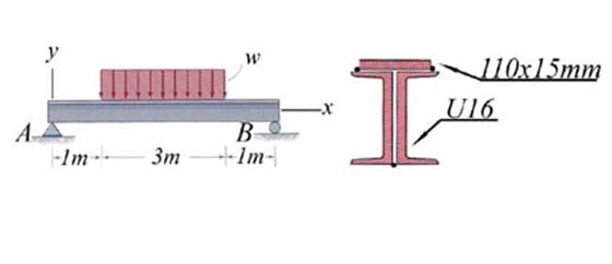
Figure 3.48
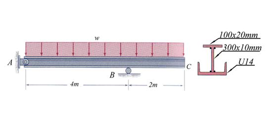
Figure 3.49
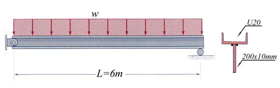
Figure 3.50
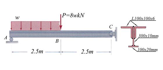
Figure 3.51
Problem 3.52 Two wood boards are attached together by screws that are spaced at regular intervals of 10 cm along the length of the beam to form the inverted tee beam shown in Figure 3.52. Each screw has an allowable shear capacity of 2 k N. Calculate the maximum allowable load P?
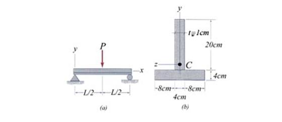
Figure 3.52
Problem 3.53
An inverted structural steel tee beam with dimensions shown in Figure 73.53 is
subjected at end C to a concentrated
force P. What is the maximum load P assuming a material with allowable
stresses of ![]() and ? Repeated the calculation for the case when the allowable
flexural tensile and compressive stresses are
and ? Repeated the calculation for the case when the allowable
flexural tensile and compressive stresses are ![]() and
and ![]() , respectively. Draw the stress distributions corresponding
to cross-section located at the left of point B. Size the welds if
, respectively. Draw the stress distributions corresponding
to cross-section located at the left of point B. Size the welds if ![]() .
.
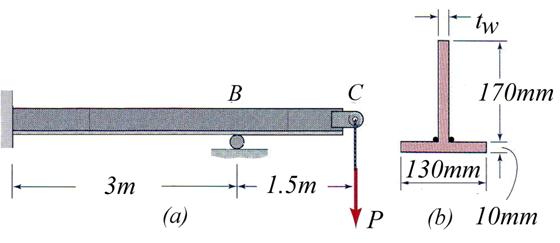
Figure 3.53
Problem 3.54 Repeat the calculations required at problem 3.53 considering the beam shown in Figure 3.54.
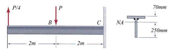
Figure 3.54
Problem 3.55
The simply supported beam, shown in Figure 3.55, has a rectangular cross-section.
Consider for the wood the following allowable stresses: ![]() ,
, ![]() and
and ![]() . Calculate: (a) Ps,
based on allowable flexural stress, (b) Pt, based on an
allowable shear stress and (c) the ratio Ps
/ Pt of the previously calculated loads. Discuss the
implications of the beam dimensions (calculate the length L for which the
shear-stress or the flexural stress criterion governs).
. Calculate: (a) Ps,
based on allowable flexural stress, (b) Pt, based on an
allowable shear stress and (c) the ratio Ps
/ Pt of the previously calculated loads. Discuss the
implications of the beam dimensions (calculate the length L for which the
shear-stress or the flexural stress criterion governs).
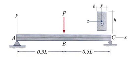
Figure 3.55
Problem 3.56
A timber beam, with 15cm x 25cm
nominal dimensions is supported and loaded as shown in Figure 3.56. If the
allowable flexural and shear stresses of the wood are: ![]() ,
, ![]() and
and ![]() , calculate the maximum load P possible to be applied to
this beam.
, calculate the maximum load P possible to be applied to
this beam.
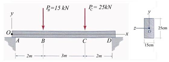
Figure 3.56
Problem 3.57 As pictured in Figure 3.57, a set of wheels on the one-axle railway car passes directly over one of the cross ties. If it is assumed that the load exercised by each wheel is represented by a uniformly distributed load pw = 500 kN/m applied over the 0.3m width of the tie plate and the cross tie distributes this load as a uniformly distributed pressure pb to the ballast on which the cross tie rests, calculate: (a) the distributed load pb, (b) the maximum shear stress, in the wood cross tie and (c) the maximum flexural stress.
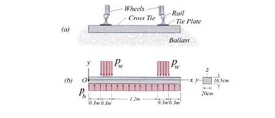
Figure 3.57
|
Politica de confidentialitate | Termeni si conditii de utilizare |

Vizualizari: 2630
Importanta: ![]()
Termeni si conditii de utilizare | Contact
© SCRIGROUP 2026 . All rights reserved