| CATEGORII DOCUMENTE |
| Bulgara | Ceha slovaca | Croata | Engleza | Estona | Finlandeza | Franceza |
| Germana | Italiana | Letona | Lituaniana | Maghiara | Olandeza | Poloneza |
| Sarba | Slovena | Spaniola | Suedeza | Turca | Ucraineana |
Data Acquisition with LabVIEW in the Multidisiplinary Engineering Laboratory I Course
Introduction
(start of Experiment I-B reading)
LabVIEW is a registered trademark of National Instruments Corporation. Parts of the following information are based on the LabVIEW Help on-line documentation. This information is copyright copyrighted by National Instruments Corporation. The authors received prior written consent of the National Instruments Corporation to use the material in this manual for the CSM MEL I Course.
Experimenters collect data from their experiments. We can gather data with instruments like a voltmeter, write the numbers into a lab notebook, and type it into a spreadsheet for analysis and graphing. However, it is much less time consuming and accurate to automatically enter the data into a file that the spreadsheet program can read and to view the data graph as we are collecting the data rather than after the experiment is completed. Therefore we use a computer data acquisition system.
The block diagram in Figure DAS-1 shows the basic components of a computer data acquisiton system. As explained in Experiment 1-B, a transducer converts the physical property, like temperature, to an electrical signal. The signal-conditioning module performs various functions like filtering, amplifying, isolating, transducer excitation, and linearization. The conditioned signal is sent to the data acquisition card that is mounted internally in our computers. The data acquisition card converts the analog voltage signal to digital values. Because it only converts voltage signals, the signal conditioning module converts the physical property value to a voltage value. The data acquisition card has other capabilities like digital to analog conversion, counter/timer circuits, and digital I/O ports. The National Instruments, NIDAQ, drivers allow the data acquisition board to communicate with and store the binary information in the computer. The National Instruments LabVIEW software provides the capability to process and display the data.
Figure DAS-1. Data Acquisition System (Portions Courtesy of National Instruments)
Experimenters can develop programs in C or BASIC to convert the analog signals to digital values and write them to files, display graphical controls and graphs on the monitor, analyze the data, etc. Text-based programming is time consuming and experimenters like to focus their time on the experiment and not programming. LabVIEW reduces the time to develop and debug data acquisition programs with a graphical programming language, G, to create programs in block diagram form. In addition to being graphical LabVIEW has extensive libraries of functions for data analysis, data presentation, and data storage. LabVIEW also includes conventional program development tools, so you can set breakpoints, animate the execution to see how data passes through the program, and single-step through the program to make debugging and program development easier.
LabVIEW
programs are called virtual instruments (
In addition
to the interactive user interface (front panel) and dataflow (block) diagram
that serves as the source code, the VI supports heirarchial programming by
using icon connections that allow the VI to be called from higher level
Front Panel
The Front Panel of a VI is a graphical user interface (GUI). The MEL I Thermistor VI Front Panel is shown below.
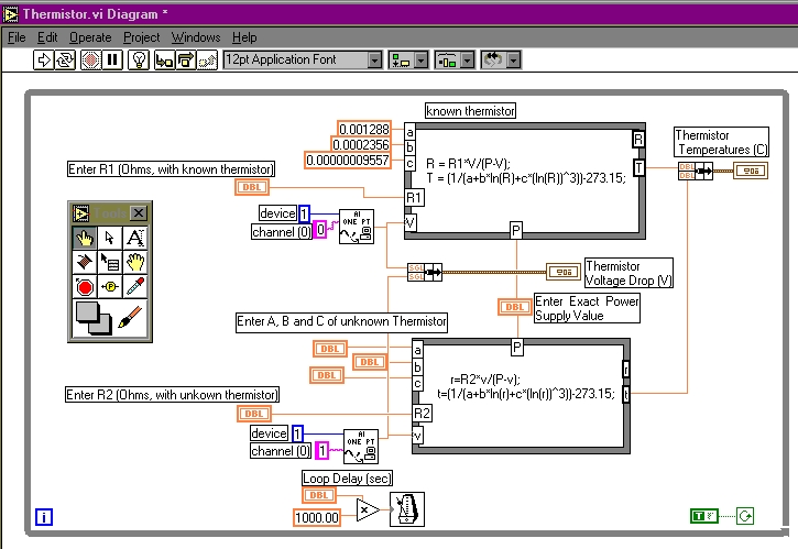
Figure DAS-2. MEL Thermistor VI Front Panel
This front panel is a combination of controls and indicators. Controls simulate instrument input devices and supply data to the block diagram of the VI.
Controls
The loop delay knob is a control that determines the delay between loops in the G program. In this program, each channel is sampled once when the loop executes, so the delay essentially controls the time delay between data samples. Temperature doesnt change quickly, so sampling quickly would just fill up the memory and computer disk with useless information, and complicate the data analysis task. The delay should be set so important data is not skipped, but to limit the number of data points.
Other controls are Enter Exact Power Supply Value, Enter R1, and Enter R2. These values should be measured with the multimeter so exact values are used in the formula that converts the voltage drop across the thermistor to temperature.
After you run the experiment and determine the coeficients of the unknown thermistor, you can use another control, enter A, B, C of the unknown thermistor, to repeat the experiment to check your results.
When building a new VI or modifying an existing one, you add controls to the front panel by selecting them from the floating Controls palette shown in the MEL Thermistor VI Front Panel. After the VI is programmed, the controls pallet can be removed. It can be added again easily if needed. You can change the size, shape, and position of a control or indicator. In addition, each control or indicator has a pop-up menu you can use to change various attributes or select different options. You access this pop-up menu (or pop up on this menu) by clicking on the object with the right mouse button.
Indicators
Indicators
simulate instrument output devices that display data acquired or generated by
the block diagram of the VI. The MEL Thermistor VI has two waveform charts that
plot thermistor temperature and voltage drop. The waveform chart displays one
or more plots, so we can plot data from a thermistor whose coefficients are
known along with an unknown-coefficient thermistor or several unknown
thermistors. Note that each chart has a legend showing the line color
associated with each thermistor data stream. Charts are different from graphs
in that charts retain previous data, up to a maximum which you can define. New
data is appended to the old data, letting you see the current value in context
with previous data. Note that each chart has a digital display that shows the
value of the current data point. Remember we said previously that
Note that there is another floating palette, the Tools Palette, shown on the Front Panel. Select the hand pointer tool to operate the VI with the run arrow on the Top Menu bar. The Top Menu bar is shown below. The icon is at the right end of the menu bar in both panel and diagram windows and is the graphical representation of the VI when it is used as a sub-VI in a larger VI.
Figure DAS-3. LabVIEW Top Menu Bar
Starting LabVIEW
You can
start LabVIEW by double clicking on the desktop icon for LabVIEW or for the MEL
I library, from the Start Programs pop up menus, or from the Windows Explorer.
If you dont start from the MEL I icon, the initial LabVIEW window asks if you
want a new VI (if you want to write a new VI in G) or to open an existing VI.
We have provided a set of
Running a VI
After
wiring your inputs to the correct pins (or channels) on the terminal block (see
the Connector Block Pin Outs Reference Sheet in this manual), click on the Run
Button (The run arrow is the right facing arrow on the menu bar shown above) to
execute the Thermistor VI. We use loops to obtain multiple data samples in MEL,
so you shouldnt have to use the continuous run button (located just to the
right of the Run Button). The Stop Button is the Red Button to the right of the
Continuous Run Button (two buttons to the right of the Run Button). We also
include stop controls in many of the Front Panels of the MEL VIs. Please stop
all
Block Diagram
The Thermistor VI underlying program in G, or the Block Diagram, is displayed in the diagram window below. It was constructed by wiring together objects that send or receive data, perform specific functions, and control the flow of execution.
Figure DAS-4. MEL Thermistor VI Block Diagram
Note that the Front Panel previously shown has a gray background, and the diagram has a white background. To display the panel or diagram, go to the menu bar and click on 'windows' pull down menu and select the window to be displayed. Both can be made full screen or you can view both simultaneously by clicking on 'tile left and right'. You can also switch from panel to diagram by pressing ctrl-e. The bottom menu bar buttons can also be used to shift between panel and diagram.
The Thermistor Diagram contains the usual VI primary block diagram program objects--nodes, terminals, and wires. When you place a control or indicator on the front panel, LabVIEW places a corresponding terminal on the block diagram. You cannot delete a terminal that belongs to a control or indicator. The terminal disappears only when you delete its control or indicator on the front panel. Terminals as entry and exit ports. Data that you enter into the controls exits the front panel and enters the block diagram through the control terminals. Note where the front panel control information, like values for the power supply, R1, and R2 enter the block diagram shown above.
Data also enters the block diagram from the data acquisition board. By connecting wires from the thermistor terminals in your circuit to the terminals on the terminal block and energizing the circuit, you supply analog voltages to the data acquisition board. The data acquisition board digitizes the voltages, and if programmed to do so enters the data into a VI. We added the AI Sample Channel Sub VI written by National Instruments in the Thermistor VI to add the data from the terminal block to the Block Diagram. The AI Sample Channel Sub VI is a Node in the program. Nodes are program execution elements. They are analogous to statements, operators, functions, and subroutines in conventional programming languages. Data enters the node, in this case from the data acquisition board, and two constants. The blue number 1 identifies the board (we only use one data acquisition board in MEL, so this number will always be 1) and the pink character 0 or 1 identifies the analog input channel (Our boards support several channels so these numbers will vary throughout the course). The node executes its subprogram (you can see the subprogram elements by expanding it with a double click) and produces new data values that exit through its terminals to other program elements.
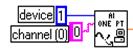
Figure DAS-5. AI Sample Channel Sub VI Icon
LabVIEW has an extensive library of functions for math, comparison, conversion, I/O, and more. Another type of node is a structure. Structures are graphical representations of the loops and case statements of traditional programming languages, repeating blocks of code or executing them conditionally. LabVIEW also has special nodes for linking to external text-based code and for evaluating text-based formulas.
Wires are the data paths between source and sink (destination) terminals. You cannot wire a source terminal to another source nor can you wire a sink terminal to another sink. You can wire one source to several sinks. Each wire has a different style or color, depending on the data type that flows through the wire. Notice that the wire from the AI Sample Channel Sub VI branches after it exits the node. One branch goes to a formula node where the voltage data is converted to temperature with a series of equations and the other branch goes to the icon for the waveform chart which plots the unconverted voltage data on the Front Panel.
Note the orange rectangles that provide data to the formula node in addition to the Sub VI and Front Panel Controls. The orange rectangles with a number inside them are constants, assigned by the author of the VI to represent the coefficients of the known thermistor.
The principle that governs LabVIEW program execution is called data flow. Stated simply, a node executes only when all data inputs have arrived; the node supplies data to all of its output terminals when it finishes executing; and the data passes immediately from source to sink (or destination) terminals. Data flow contrasts with the control flow method of executing a conventional program, in which instructions are executed in the sequence in which they are written. Control flow execution is instruction driven. Dataflow execution is data driven or data dependent.
Wired logic is different from other languages. The wired connections persist for the life of the program and cannot be modified during execution. In most languages one can write x=y at one point and later write x=z. This is not possible in LabVIEW and x remains equal to y for the entire program.
The Formula Node is a control structure. A LabVIEW control structure is a subroutine. It is receives inputs, performs some job and returns outputs. The job may take a long time and include other VI's and control structures. The control structure may change items on the panel and it may accept operator input from the panel. LabVIEW has 5 types of control structures: FORMULA, WHILE, FOR, CASE and SEQUENCE. A control structure has an inside and an outside separated by a thick border. The code inside the border is referred to as a sub-diagram. Variables go through the border via tunnels, small rectangles in the border.
The FORMULA structure provides a compact way to express mathematical relationships between inputs ( thin edged rectangles on the border ) and outputs ( thick edged rectangles on the border) in the Thermistor VI Block Diagram. The relationships are defined by C language statements in the sub-diagram. National Instruments provides a library of math functions which can be included in the C language statements. You will notice that the structure can use intermediate variables, not wired to other nodes. As stated above, we passed constants as inputs to the FORMULA structure, but they can also be written into the equations.
Printing a Window
To print a Front Panel or Block Diagram Window, choose the File pull down menu from the Top Menu Bar and select print window. (The hot key is cntrl P.)
LabVIEW On-Line Help
MEL is about learning how to learn. Through using LabVIEW, studying this reference, and using the LabVIEW on-line help you will learn about LabVIEW. However, in the future, you may use a different version of LabVIEW, or different data acquisition software. Therefore, it is essential that you become comfortable with on-line help to continue to learn on your own in the future.
The Help window contains help information for functions, constants, subVIs, controls and indicators, and dialog box menu items. To display the window, choose Show Help from the Help menu located on the Top Menu Bar or press <Ctrl-h> (Windows). Move your cursor over the icon of a function, a subVI node, or a VI icon (including the icon of the VI you have open, shown at the top right of the VI window) to see the help information.
Selecting HelpLock Help or clicking on the lock icon at the bottom of the window locks the current contents of the Help window. When you lock it, moving over another function or icon does not change the display in the Help window. Select Lock Help or click on the lock icon again to turn this menu item off.
The Help window displays the most commonly required help information in a condensed format. To access more extensive online information, select Help Online Reference. For most block diagram objects, you can select Online Reference from the pop-up menu of the object. You also can access this information by pressing the ? button, which is located at the bottom of the Help window.
Instead of using Show Help from the Help Menu, you can choose On-Line Reference. You can search for a particular topic or browse the topic list.
Note that a LabVIEW reference sheet explaining the various icons is included at the end of this Reference Section.
(end of Experiment I-B reading) (start of Experiment 2-A reading)
You can
select some properties of the control and indicator objects. LabVIEW has what National
Instruments calls PopUp Menus for most objects. To access a PopUp, right click
on the object. These menus are useful guides to the methods associated with
LabVIEW objects and you should get in the habit of right clicking on things
just to see what they can do. All of the
Numerical data: Integer and Floating Point representations
LabVIEW numbers come in two varieties: integer and floating point. Notice the difference between the colors used in the Strain Gage Bridges VI diagram for the bridge type (integer - blue) and the supply voltage (floating point - orange). LabVIEW will sometimes convert one type to another and indicates the conversion in the diagram by placing a small dot at the wire terminal where the conversion occurs. Try changing the weight indicator to an integer representation to illustrate a numerical conversion.

Figure DAS-6. Portion of the Strain Gage Bridges VI Block Diagram
Palettes
Editing a LabVIEW program uses three floating 'palettes', windows with icons which can be positioned anywhere on the screen. To display a palette, click on windows on the menu bar and then click on show palette. In MEL I, you will primarily use the tools palette which contains mouse pointers with specific properties for different jobs. The various tools are defined in the LabVIEW Reference Sheet in the Reference Section of this manual. For instance, the hand pointer is used to manipulate panel controls while the arrow pointer is used to select and drag objects.
In MEL I, we wont use the controls and function palettes often, but just so you know what they are in case you want to use them: The controls palette contains panel objects. To place an object on the panel, click on a family box, like string and table, and then click on a control or indicator. Finally, move the dotted outline of the indicator to its panel location and click to place the object. The function palette is a collection of built-in subroutines for use in the diagram. This palette also accesses sub-VI's from National Instruments or one that you might write. Selection and placing a function on the diagram is done in a fashion similar to the control palette.
CASE Structure
The Strain Gage Bridges VI Block Diagram contains a CASE control structure. Case structures can have multiple subdiagrams, configured like a deck of cards, of which only one is visible at a time. Only one subdiagram runs at a time. An input or selector determines which sub diagram executes. At the top of each structure border is the subdiagram display window, which contains a diagram identifier in the center and decrement and increment buttons at each side.
Clicking the decrement (left) or increment (right) button displays the previous or next subdiagram, respectively. Depending on the input to the structure, one of several subprograms may be run. For example, the CASE structure can be used like an IF THEN statement in a text programming language. If you input a 1 (representing TRUE) a sub diagram will execute and you can leave the 0 (representing FALSE) empty. The CASE structure in the Strain Gage Bridges VI Block Diagram has 3 sub-diagrams, labeled 0,1 and 2 for the different equations to calculate strain from output voltages in 1,2, and 4 gage bridges. The user determines which equation executes by selecting the proper bridge type from the control on the Front Panel.
The CASE structure may have sub-VI's and timed functions within its sub-diagrams. Unlike the FORMULA structure, a CASE structure can take a long time to execute. Remember that the inputs to control structures are evaluated only once, when the structure begins execution.
Numeric Functions
The Strain Gage Bridges VI Block Diagram uses wired logic and a simple math function from the numeric family of the function palette to implement the software multiplier. When you have LabVIEW open, look at the numeric functions, which are available. They include complex trigonometric and array functions, a random number generator and numeric constants. LabVIEW functions are polymorphic; that is, they will adapt the operation to the types of inputs that are wired to the function.
(end of Experiment 2-A reading)
Working with LabVIEW and Excel
(Start of Experiment 2-B reading)
Many times it is convenient to open LabVIEW and EXCEL simultaneously at the lab bench computers. This is particularly true if you need to analyze data as required in Experiment 2. If you haven't used multiple programs simultaneously in Windows (multitasking) before take the 10-minute tour, from the Windows 95 or NT desktop, click the start button, click help, and click on the 10-minute tour. Look at starting programs and switching windows.
When you run the LabVIEW VI for Experiment 2, it will ask if you want to save the data, and it will query you for a file name per the Write to Spreadsheet ?File Sub VI in the Block Diagram below. If you are at a point in the experiment where you want to save data, choose 'yes'.
YOU SHOULD SAVE THE DATA IN TWO PLACES IN CASE A DISK FAILS. SAVE IN C:TEMP AND ON ONE OR MORE FLOPPY DISCS. YOUR TEAM SHOULD KEEP TWO FLOPPY DISCS DIVIDED BETWEEN TEAM MEMBERS WITH ALL OF YOUR FILES FOR THE MEL I COURSE, SO IF ONE DISC IS DAMAGED OR THE PERSON WHO HAS THAT DISK DOESN'T ATTEND, YOUR WORK WILL NOT BE IMPEDED.

Figure DAS-7. Save to File Portion of Strain Gage Bridges VI Block Diagram.
Write to Spreadsheet Function
LabVIEW provides a function which can create a spreadsheet file of rows and columns of numbers, displayed as characters, which can be input to spreadsheet programs. When this file function begins execution, the first item to appear will be a standard windows file dialog. You will be able to type in the name which you want to use for the data file and where it should be stored. Remember, the MEL labs can only use C:TEMP or A: for data storage. After the file dialog, the file is written and the main VI terminates. If you abort the VI, you will not always get to the file writing function. The spreadsheet file is an ASCII text file with spaces for delimiters and must be 'imported' into the spreadsheet program, it is not an actual spreadsheet file. If you like, you can view the file with a word processor like NotePad.
The Write to Spreadsheet File Function actually converts a 2D or 1D array of single-precision (SGL) numbers to a text string and writes the string to a new byte stream file or appends the string to an existing file. You can optionally transpose the data. If you dont transpose it, the function writes the numbers in rows rather than columns. This sub VI opens or creates the file before writing to it and closes it afterwards. You can use this sub VI to create a text file readable by most spreadsheet applications. This sub VI calls the Array to Spreadsheet String function to convert the data.
After you save the data, open that file in EXCEL. If you havent imported data into a spreadsheet like EXCEL before,to get instructions on importing data, start EXCEL, open Help, and find importing data, text files. Read this portion of the EXCEL help information and then use the wizard that opens when you import the data. The wizard assists you in dividing multiple column data into correct columns in the spreadsheet.
Dialog Boxes
When the main WHILE loop is terminated, two pieces of data are output through the two 'tunnels' in the right side of the WHILE loop in the above block diagram. One is the data array and the other the answer to the question of whether or not to save the data. The dialog question is generated when the loop stops execution by the dialog box sub VI that is located just outside and right of the loop. This is a LabVIEW function which displays a standard windows dialog box. The program waits until the operator clicks on one of two buttons.
String Data
A string is a sequence or array of characters. LabVIEW does not attach any numeric value or meaning to the sequence. There are special functions for handling strings and their wires and panel objects are colored pink. Note that in the previous Figure DAS-5. AI Sample Channel Sub VI Icon, the channel is specified with a string. For this lab, the string contains one character, 0, but it could contain a string like '2,5,9' which would cause samples to be taken from 3 analog inputs at each sample timing interval.
Notice that the Dialog Box in Figure DAS-7 contains String Data that is written to the Front Panel to query the user about whether this data should be saved. The combination of the dialog box and the case structure (save if TRUE) allows the user to just save good data. That is, if there was an experimental error and the data is invalid, the experiment can be repeated without filling up the storage media with unnecessary files.
Customizing Charts and Graphs in LabVIEW
Study the LabVIEW Reference Help on Graph and Chart Controls and Indicators: Graph Options and experiment with the following to improve the appearance and readability of your graphs in the VI. Many of these features are accessible from the graph pop-up menu and its submenus.
Printing a Graph
There are several options:
Use option 1 if you just need to print the Front Panel. Use option 2 if you want to save the Front Panel as a .BMP and print is elsewhere. Use option 3 if you have to print information other that that on the front panel, for example Output Volts vs. Force ( the panel displays Output Volts vs. Sample Number).
(end of Experiment 2-B reading)
Acquiring Multiple Samples Of A Voltage Waveform
(Start of Experiment 3 reading)
The Block Diagram of the Snapshot VI is shown below in Figure DAS-8. The hardware interface in this VI is performed by a National Instruments sub-VI called AI Acquire Waveform and labelled 'AI mult pt' in the icon. It acquires a specified number of samples at a specified sample rate from a single input channel and returns the acquired data. When it is executed, this VI performs many a/d conversions on a single channel. In addition to inputs specifying the data acquisition board and the channel, this sub-VI has an input for the total number of samples to be taken and the rate at which the voltage is to be sampled. The output from this VI is two wires: the thin one carries the sample period (seconds between successive samples) and the thick one carries 600 numbers, one for each voltage sample which was acquired.
The main difference between the Analog Input Sub VI, AI Sample Channel, used in previous experiments is that the AI Acquire Waveform Sub VI performs a timed measurement of a waveform (multiple voltage readings at a specified sampling rate). This wasnt necessary in the thermistor or force transducer experiments, because precise time data wasnt relevant to the measurements required. However, in the oscillation experiment precise times are necessary to measure period and frequency. In addition, high sampling rates were not necessary in previous experiments, and we even inserted delays in the block diagrams loops. The Acquire Waveform Sub VI sample timing is done by hardware located on the data acquisition board. Voltage sample data is stored in the computer's memory using direct memory access (DMA). The sampling can be done at high rates, up to 100,000 samples per second. If sampling two channels, each channel can be sampled at 50,000 samples per second. In comparison, when sample acquisition timing and storage are controlled by software, as with the AI Sample Channel Sub VI, the maximum rate is about 100 samples per second.
BEWARE; AI Acquire Waveform Sub VI does not respond to the abort button when the sub-VI is gathering data. If you select 10,000 samples at 1 sample per second, you will have to wait a long time or reset the computer. If you select no samples or a sample rate beyond the capability of the board, you will get an error message. Think carefully about how fast you want to sample, and how many samples you want to take.

Figure DAS-8. Snapshot VI Block Diagram.
Clusters
The array of data, the sample period and a start time equal to 0.0 are sent to a function which combines them into a single element of a new type of data, the cluster. A LabVIEW cluster is an ordered list of simple data elements, possibly of different types. The cluster is a programmer defined data type. It can be sent along wires and connected to terminals in the same manner as simple data. Note the color and patterned wire used for the cluster. Generally, they are used as a wiring and organizational convenience. The function or sub-VI to which they are wired must be programmed to use the particular cluster with the exact number of data types in the proper order. For this VI's cluster, we have combined three streams of data to supply the information needed to create a graph. The information includes the minimum x value ( 0.0 ), the step size on the x axis ( the sample period ) and the y values to be associated with each x axis point (the data array from the sub-VI ).
Waveform Graphs
The Snapshot VI uses the waveform graph rather that the waveform chart that was used in previous experiments. A graph is a two-dimensional display of one or more data arrays called plots. The difference between a graph and a chart is that a graph plots data as a block, whereas a chart plots data point by point, or array by array.This produces a 2 dimensional plot of an array of ordered ( x,y ) pairs. Multiplot graphs with several y values for each x value can also be created. The x axis spacing must be uniform. The data to be input to the graph must be the complete set of points; you cannot incrementally add a point to a graph like you can with the chart. The x and y axis range can be computed by LabVIEW when the graph is plotted or you can change the ranges with the operating tool, by clicking on and editing the maximum or minimum value on the graph axis. In the upper right is a legend which identifies the different plots in a multiplot graph. At the lower left is a palette with tools to autoscale the x and y axis, zoom in to a point and pan the graph. The graph also has a cursor palette. PopUp in the middle of the graph's screen to select which palettes are to be visible and to change the format of the axis labeling. You can choose various grid styles and logarithmic y-axis scales. (Refer to the previous information on Customizing charts and Graphs in LabVIEW.
(End of Experment 3 Reading)
Array Data
(Start of Experiment 4 Reading)
Since MEL I, Experiment 4 VI integrates thermal and strain measurement, the Thermal Coefficient VI combines the two data streams with time data in an array as shown in Figure DAS-8. Snapshot VI Block Diagram, below. An array is an ordered list of similar data elements. You can have arrays of any simple data type like integers or strings. An array control or indicator contains two parts: the data elements and an index display. The index denotes the position of an element in the list. The first element has an index = 0. An array is usually displayed as a row or column of numbers. Arrays can have multiple 'dimensions'. A 2D array, for instance, would be displayed as several rows or columns of numbers and each element would have a row index and a column index. Normally, the indexes are listed in (column, row) order.
Note that two channels of data from the A/D board go to two different formula nodes, one to convert thermistor voltage drop to temperature and the other to convert the strain gage bridge output voltage to strain. Then these two data streams are inputs, along with time, to a build array node. The output from the build array node is wired to a Write to Spreadsheet File Sub VI. There are actually two arrays formed in this sequence. The first ( 1D ) array is formed by the 'build array' function which creates a three column array of temperature, strain, and time data. Note the thickness of the wire for the 1D array. The second ( 2D ) array is created when the voltage data tunnels through the border of the loop. This creates a 3 column by N row output array (where N is the number of times the loop executes). Note the double wire for the 2D array.
The wires from thermistor and strain gage circuits to the Terminal Block Pins must agree with the channel numbers in the Thermal Coefficient Block Diagram. That is, the thermal data must enter channel 0 and the strain data must enter channel 1. If they are reversed, the thermal equations would be applied to the strain data.
Also notice that data streams of thermal and strain voltages and engineering units are displayed in four waveform charts on the Front Panel.

Figure DAS-8. Snapshot VI Block Diagram.
While Loop
The main control structure in this VI is a new one, the WHILE loop. This looping structure repeatedly executes the code in the sub-diagram until the boolean connected to the termination control in the lower right corner becomes false. Any Boolean variable can be used as the termination control.
The iteration count in the lower left corner is zero when the loop begins and is incremented each time the sub-diagram executes. Inputs to the WHILE loop are evaluated at the first iteration and these values are used over and over again for all succeeding iterations. Outputs from the WHILE loop are the ones which resulted from the actions taken during the last iteration.
Shift Register
The WHILE loop has a kind of local memory called a 'shift register'. It's graphical representation is an upward pointing arrow in the right border ( the output ) and a downward pointing arrow in the left border ( the input ). The shift register saves a computed result from the current iteration and makes it available as an input for the next iteration. The first iteration can use an initial value from outside the WHILE loop. In the Thermal Coefficient VI, the shift register output combines with the time delay in the loop to detemine the time elapsed between samples and enter it in the array.
Timing
A small metronome has been included near the bottome of the WHILE Loop in this and several of the previous VIs. It is the icon for the Wait Until the Next ms Multiple' Sub VI. It waits until the value of the millisecond timer becomes a multiple of the specified millisecond multiple. It is used to control the loop execution rate. However, it is possible that the first loop period might be short.
Boolean Variables and Controls
In the Thermal Coefficient VI we an End VI, Red Stop Button on the Front Panel. This is a preferrble way to the Abort Button on the Top Menu Bar of terminating execution of VIs. Many of the VIs used in previous experiments, like this one, have a 'Save to File?' dialog which is another example of a Boolean Control. Booleans are two value variables: true or false, on or off, active or inactive, zero or one. They are represented by lamps and pushbuttons on the panel. True lamps are on and true buttons are pressed inward or are in the up position. Boolean variables are the outputs from comparison functions like 'is x greater than y'.
(End of Experiment 4 Reading)
A/D Board Gain
(Start of Experiment 5 Reading)
The Pressure VI Block Diagram below illustrates another feature of the DAS Amplification. The full scale output of the Omega PX236 Pressure Transducer is 60mv. With a digitizing resolution of 4mv, pressure readings would not be very precise. However this poor resolution occurs when the board is configured for 10V full scale. By reducing the maximum voltage, we can apply the 12 bit resolution over a smaller range, effectively amplifying the signal per the following table.
Note that the AI Sample Channel Sub VI in the Pressure VI Block Diagram below has a wire connecting to a Front Panel Control to set the maximum input voltage. If we set it at 100 mV, we achieve a gain of 100, considerably improving the digitizing resolution for the 60 mV Omega Pressure Transducer output.
Figure DAS-9. Pressure VI Block Diagram.
|
Actual Input Range |
Gain |
Digitizing Resolution |
|
0 10 V |
2.44 mV |
|
|
0 5 V |
1.22 mV |
|
|
0 2 V |
m V |
|
|
0 1 V |
m V |
|
|
0 500mV |
m V |
|
|
0 200mV |
m V |
|
|
0 100mV |
m V |
Table DAS 1. DAS Variable Gain (Modified from National Instruments)
(End of Experiment 5 Reading)
Power Spectrum
(Start of Experiment 6 Reading)
Refer to 'Frequency Domain, Power Spectra, and Signal Sampling' section of this reference for an explanation of frequency spectrum graphs. The samples of a signal obtained from a DAQ board constitute the time domain representation of the signal. This representation gives the amplitudes of the signal at the instants of time during which it had been sampled. However, in many cases you want to know the frequency content of a signal rather than the amplitudes of the individual samples. The representation of a signal in terms of its individual frequency components is known as the frequency domain representation of the signal. The frequency domain representation could give more insight about the signal and the system from which it was generated.
The algorithms used to transform samples of the data from the time domain into the frequency domain is known as the fast Fourier transform (FFT) or discrete Fourier transform (DFT). They establish the relationship between the samples of a signal in the time domain and their representation in the frequency domain. They are widely used in the fields of spectral analysis, applied mechanics, acoustics, medical imaging, numerical analysis, instrumentation, and telecommunications.
The plot showing the power in each of the frequency components is known as the power spectrum. The Power Spectrum VI in the AnalysisDigital Signal Processing subpalette calculates the power spectrum of time domain data samples. It is implemented in two MEL I VIs: Figure DAS-10, Continuous 1024 Hz with FFT VI Block Diagram, and Figure DAS-11, the Snapshot with FFT VI Block Diagram.
When the number of samples and the sampling rate are a power of 2, the Power Spectrum Vi uses the FFT. The FFT computation of the Power Spectrum is extremely fast and memory efficient because the transform is real and done in the same space. However, the size of the input sequence must be exactly a power of 2. If the number isnt a power of 2, the Power Spectrum uses the DFT. The DFT version efficiently computes the Power Spectrum of any size sequence. The DFT version is slower than the FFT version, uses more memory, and is not as efficient in scaling. Therefore, both FFT VI block diagrams shown below use power of 2 sampling.
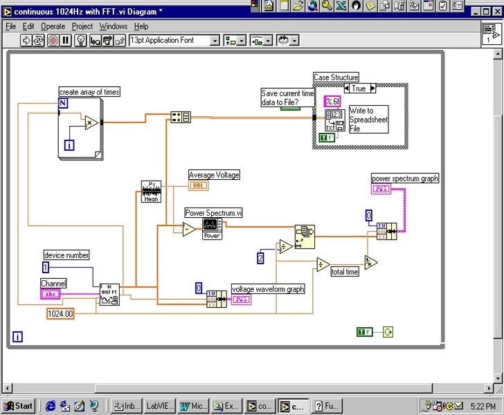
Figure DAS-10. Continuous 1024 Hz with FFT VI Block Diagram
The Continuous 1024 Hz with FFT VI Block Diagram contains a FOR Loop. A For executes its subdiagram count times, where the count equals the value contained in the count terminal. You can set the count explicitly by wiring a value from outside the loop to the left or top side of the count terminal, or you can set the count implicitly with Auto-Indexing. The other edges of the count terminal are exposed to the inside of the loop so you can access the count internally.
The iteration terminal contains the current number of completed iterations; 0 during the first iteration, 1 during the second, and so on up to N 1. Both the count and iteration terminals are signed, long integers.

Figure DAS-11. Snapshot with FFT VI Block Diagram
Execution order and Multitasking
The graphical appearance of loops within sequences within other structures is common in LabVIEW. Execution begins with the innermost control structure. When an inside structure is complete, the surrounding one is begun.
LabVIEW is a multitasking operating system. At any moment, there may be several active nodes (functions and sub-diagrams). The code for all of them is executed simultaneously. When one node's work is complete, it is removed from the active list and its output data sent downstream to another node. If the downstream node has all of its inputs available, it is added to the active list. Normally, the only control on the order of execution is by wiring. This is a very different situation from most languages which have an strongly enforced execution ordering in the source code line sequence.
SEQUENCE Structure
The SEQUENCE structure is LabVIEW's mechanism to enforce the order of execution,
and you will find one inside the WHILE loop of the Snapshot FFT VI. The Sequence Structure, which looks like a frame of film, consists of one or more subdiagrams, or frames, that execute sequentially. Determining the execution order of a program by arranging its elements in sequence is called control flow. BASIC, C, and most other programming languages have inherent control flow, because statements execute in the order in which they appear in the program. The Sequence Structure is a way of obtaining control flow when data dependencies are not sufficient. A Sequence Structure executes frame 0, followed by frame 1, then frame 2, until the last frame executes. Only when the last frame completes does data leave the structure.
Within each frame, as in the rest of the block diagram, data dependency determines the execution order of nodes. Tunnel inputs to the structure are evaluated when the first frame begins execution, even if the input is wired to something in a later frame. Tunnel outputs from the structure are available when the last frame finishes, even if they were computed in an earlier frame. Panel controls which appear within a frame are read or updated when the frame executes.
LabVIEW Triggering
Sometimes it is good to begin data acquisition and graphical displays on the VI based on the condition or state of incoming analog or digital data. For example, in experiment 6, you need to begin acquisition when oscillation begins, or when initial steady state ends. You can simultaneously click the run button when you oscillate the beam, but you might have to do it a few times before you synchronize properly. Try and see if it is difficult.
Triggering automatically starts the data acquisition process. In LabVIEW, you can trigger on an external signal that is either analog or digital, or you can use a software trigger. In experiment 6, we use analog data, so we will concentrate the explanation there.
In order to utilize triggering, you set some trigger conditions, for example when voltage begins to rise and goes beyond a certain level, or when the voltage signal begins to fall. Some DAQ devices monitor the analog channel and begins acquisition only when the conditions are met. Unfortunately, our DAQ boards do not have this capability, so we use a software trigger that simulates analog triggering. The software triggers are entered on the front panel of the VI and built into the block diagram controls as shown in the Trigger with Pretrigger and FFT VI Block Diagram below. Note that there is also a Trigger with Pretrigger VI available in the MEL I library. Essentially, the device continues to collect data, but does not send it to LabVIEW unless the trigger conditions are met.
Pretrigger scans is the number of scans you want the VI to save in the buffer before the trigger. The default input is 0, which tells LabVIEW to acquire all data after the trigger. You can override the default by setting the number of pretrigger scans with the Trigger with Pretrigger and FFT VI. The ability to collect pretrigger scans gives greater ability to capture the start of an event.
It is also possible to specify triggering on falling or rising edges or slopes with the following choices in the AI Waveform Scan Sub VI.
0: Do not change the edge or slope setting (default input).
1: Leading edge for digital trigger or positive slope for analog trigger.
2: Trailing edge for digital trigger or negative slope for analog trigger.
Users can also specify which analog channel is the source of the trigger. An empty string tells LabVIEW not to change the trigger source setting (default input).
Users can also set the level, i.e. the value the analog source must cross for a trigger to occur. You must also specify whether the level must be crossed on a leading or trailing slope using the edge or slope input. You express level in the units of your readings. The default input for level is 0.0.
Use the On-line Reference in LabVIEW for more information on triggering with the AI Waveform Scan VI.
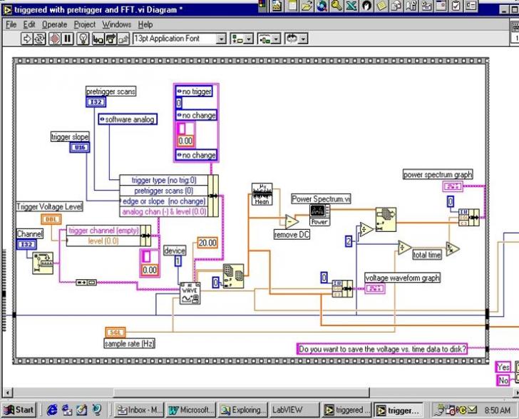
Figure DAS-12. Portion of Trigger with Pretrigger and FFT VI Block Diagram.
|
Politica de confidentialitate | Termeni si conditii de utilizare |

Vizualizari: 3731
Importanta: ![]()
Termeni si conditii de utilizare | Contact
© SCRIGROUP 2025 . All rights reserved