| CATEGORII DOCUMENTE |
| Bulgara | Ceha slovaca | Croata | Engleza | Estona | Finlandeza | Franceza |
| Germana | Italiana | Letona | Lituaniana | Maghiara | Olandeza | Poloneza |
| Sarba | Slovena | Spaniola | Suedeza | Turca | Ucraineana |
Gaussian and Other Low Lag Filters
The first objective of using smoothers is to eliminate or reduce the undesired high frequency components in the price data. Therefore, these smoothers are called low pass filters, and they all work by averaging in one way or another. I previously described the design and use of Butterworth low pass filters to achieve greater filtering than can be obtained by simple averagers. However, nothing comes for free. A higher degree of filtering is necessarily accompanied by a larger amount of lag. Thats just a fact of life.
Since lag is the downfall of most trading indicators, leading to the failure to react to price changes in a timely manner, a better approach to filtering is to minimize the lag and accept whatever smoothing results. The importance of lag is demonstrated in Figure 1, the lag of a 3 pole Butterworth filter that attenuates cycles shorter than 10 bars. We traders think in terms of cycle periods, but filter responses are usually plotted in terms of frequency. Frequency is the reciprocal of period. The frequency scale is normalized to a 2 bar cycle (the Nyquist frequency for daily data).
Figure 1. Lag of a 3 Pole Butterworth Filter with a 10 bar Period Cutoff
The low frequency lag of a Butterworth filter can be estimated from the equation
Lag = N*P / 2
Where N is the number of poles in the filter and P is the longest cycle period to be passed through the filter. The lag story gets worse as the frequency components of the input waveform are near the band edge of the filter. The higher frequency components within the passband of the filter are actually delayed more than the lower frequency components. This is exactly the opposite of what a trader desires. We have to react faster to faster changes in the market, and so we would prefer a smoothing filter that actually has less lag to the higher frequency components.
The use of Gaussian filters is a move toward the dual goals of reducing lag and reducing the lag of high frequency components relative to the lag of lower frequency components. Multipole Gaussian filters can be constructed that provide a desired degree of smoothing. The group delay of a 3 pole Gaussian filter having a .1 cycle per day passband is shown in Figure 2 for comparison to the delay produced by a Butterworth filter.
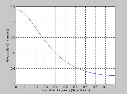
Figure 2. Lag of a 3 Pole Gaussian Filter with a 10 Bar period Cutoff
For an equivalent number of poles, the lag of a Gaussian filter is about half the lag of a Butterworth filter. More importantly, the higher frequency components have still less lag than the low frequency components. With Gaussian filters the lag as a function of frequency is going in the right direction for traders. It is also true that a Gaussian filter has about half the smoothing effectiveness as an equivalently sized Butterworth filters. Said another way, a 4 pole Gaussian filter has about the same smoothing performance as a 2 pole Butterworth filter. Thus, to do the same filtering job, these two filters would have about the same low frequency lag but the Gaussian filter would preserve the original price function with greater fidelity because the higher frequency components within the passband would not be delayed as much as in the Butterworth filter. Comparative filter responses of a 2 pole Butterworth filter and a 2 pole Gaussian filter, each having a 10 bar cycle passband, is shown in Figure 3.
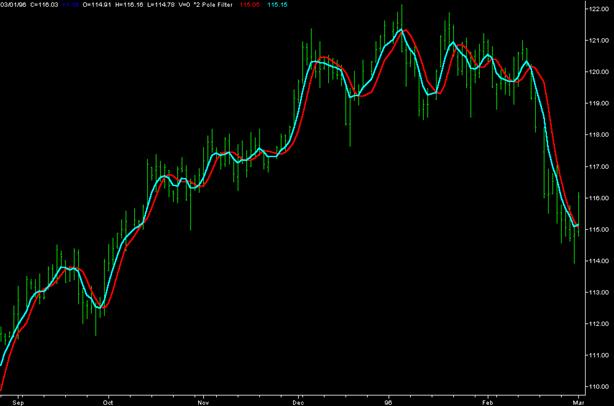
Figure 3. Comparison of 2 Pole Filters shows the Gaussian filter (Cyan)has much less lag than the Butterworth filter (Red). The Gaussian filter has less smoothing.
There is no magic to a Gaussian filter. It is just the multiple application of an Exponential Moving Average. From my previous article the transfer response of an exponential moving average is
H(z) = / (1 (1-) Z-1)
So that applying the exponential moving average N times gives a N Pole filter response as
H(z) = N / (1 (1-) Z-1)N
At zero frequency Z-1=1, so this low pass filter has unity gain. Also, the denominator assumes the value of N at zero frequency. The corner frequency of the filter is defined as that point where the transfer response is down by 3 dB, or .707 in amplitude. When this occurs, we have the relationship
(1 (1-) Z-1)NN where Z-1 = e-j and = 2/P
Crunching through the complex arithmetic, we arrive at the solution for alpha as
= - + SQR(2 + 2)
Where = (1 cos()) / (1.4142/N 1)
This generalized solution for alpha can be used to compute the coefficients for any order Gaussian filter. Recalling that the filtered output is determined by the equation
f(z) = H(z)g(z) where g(z) is the input price
If H(z) is of the form 1/(1 (1-) Z-1)N we can easily form equations for the output in EasyLanguage metaphor because Z-1 is synonymous with a one bar lag. These equations are:
One Pole: f = g + (1-)f[1]
Two Poles: f = 2g + 2(1-)f[1] - (1-)2f[2]
Three Poles: f = 3g + 3(1-)f[1] - 3(1-)2f[2] + (1-)3f[3]
Four Poles: f = 4g + 4(1-)f[1] - 6(1-)2f[2] + 4(1-)3f[3] - (1-)4f[4]
Etc.
It is often easier to go to a lookup table to get filter coefficients rather than uniquely calculate the coefficients each time they are used. In the following tables, the notation is that B is used with the price data and A is used with the previously calculated filter output [N] bars ago. I hope these tables at the end of the article make it easier to use higher order filters.
The equation for a simple 3 bar moving average is
f = .25*g + .5*g[1] + .25*g[2]
where each of the gs corresponds to the price. In terms of navigation, the g values are the values of position to compute a smoothed estimate of position. If we take a page from the book on Kalman filters and introduce a velocity term in addition to the position term we can arrive at a better smoothed estimate. So, in the above equation, let each of the price values become g + (g g[1]) = 2*g g[1]. The three bar moving average equation then becomes
f = .5*g +.75g[1] + 0 -.25*g[3]
Guaranteed you will not get much filtering out of this filter. In fact, you will probably get some overshoot. Its strength is that you can filter one of the Gaussian filter smoothed results to further reduce the higher frequency lag. Remember, that by decreasing the lag you are also decreasing the amount of smoothing that you can obtain.
|
One Pole (EMA) | ||
|
Period |
B[0] |
A[1] |
|
Two Pole | |||
|
Period |
B[0] |
A[1] |
A[2] |
|
Three Pole |
| |||
|
Period |
B[0] |
A[1] |
A[2] |
A[3] |
|
Four Pole | |||||
|
Period |
B[0] |
A[1] |
A[2] |
A[3] |
A[4] |
|
Politica de confidentialitate | Termeni si conditii de utilizare |

Vizualizari: 1062
Importanta: ![]()
Termeni si conditii de utilizare | Contact
© SCRIGROUP 2025 . All rights reserved