| CATEGORII DOCUMENTE |
| Bulgara | Ceha slovaca | Croata | Engleza | Estona | Finlandeza | Franceza |
| Germana | Italiana | Letona | Lituaniana | Maghiara | Olandeza | Poloneza |
| Sarba | Slovena | Spaniola | Suedeza | Turca | Ucraineana |
Theory of Commutation
For the successful operation of a dc machine, the induced emf in each conductor under a pole must have the same polarity. If the armature winding is carrying current, the current in each conductor under a pole must be directed in the same direction. It implies that as the conductor moves from one pole to the next, there must be a reversal of the current in that conductor. The conductor and thereby the coil in which the current reversal is taking place are said to be commutating. The process of reversal of current in a commutating coil is known as commutation.
Ideally, the process of commutation should be instantaneous, as indicated in Figure 5.12a. This can, however, be achieved only if the brush width and the commutator segments are infinitesimally small. In practice, not only do the brush and the commutator have finite width but the coil also has a finite inductance.
Therefore, it takes some time for the current reversal to take place, as illustrated in Figure 5.12b.
Figure 5.13a shows a set of eight coils connected to the commutator segments of a 2-pole dc generator. The coils g, h, a, and b are under the north pole and form one parallel path, while the coils c, d, e, and f are under the south pole and form another parallel path. The current in the coils under the north pole, therefore, is in the opposite direction to the current in the coils under the south pole. However, the magnitude of the current in each coil is Ic. The width of each brush is assumed to be equal to the width of the commutator segment. Brush A is riding on commutator segment 3 while brush B is on segment 7. The current through each brush is 2Ic. As the commutator rotates in the clockwise direction, the leading tip of brush A comes in contact with commutator segment 2 and shorts coil b as indicated in Figure 5.13b. Similarly, the coil f is also short-circuited by brush B.
The coils b and f are now undergoing commutation. From Figure 5.13b it is evident that the current through each brush is still 2Ic. At this instant, the induced emfs in coils b and f are zero because each lies in the plane perpendicular to the flux. However, an instant later, the contacts of brushes A and B with commutator segments 3 and 7 are broken as depicted in Figure 5.13c. Coil b is now a part of the parallel path formed by coils c, d, and e, and the direction of the current in the coil has reversed. Similarly, coil f has become a part of the parallel path formed by coils a, h, and g, and its current has also reversed its direction. The commutation process for coils b and f is complete. Coils a and e are now ready for commutation. In a multiple machine, the number of coils undergoing commutation at any instant is equal to the number of parallel paths when the brush width is the same as the width of the commutator segment.
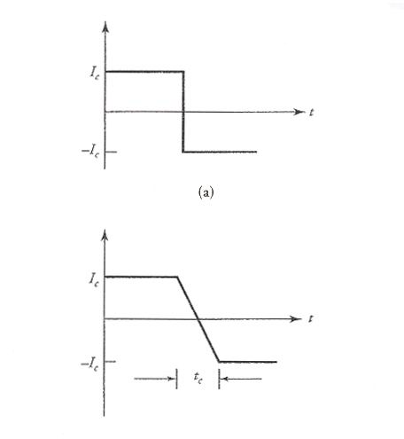
Figure 5.12 Current reversal in a coil undergoing commutation with brushes of (a) infinitesimal thickness and (b) finite thickness.
For commutation process to be perfect, the reversal of current from its value in one direction to an equal value in the other direction must take place during the time interval tc. Otherwise, the excess current (difference of the currents in coils b and c) prompts a flashover from commutator segment 3 to the trailing tip of brush A. Likewise, a flashover also takes place from commutator segment 7 to the trailing tip of brush B.
When the current reverses its direction during commutation in a straight-line fashion as illustrated in Figure 5.12b, the commutation process is said to be linear. A linear commutation process is considered to be ideal in the sense that no flashover occurs from the commutator segments to the trailing tips of the brushes. In the next section, we discuss methods that allow us to improve commutation under varying loads.
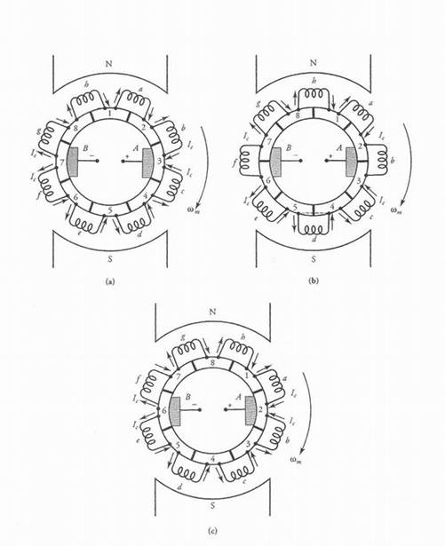
Figure 5.13 Coils b and f (a) prior to, (b) during, and (c) after the commutation process.
5.8 Armature Reaction
When there is no current in the armature winding (a no-load condition), the flux produced by the field winding is uniformly distributed over the pole faces as shown in Figure 5.14a for a 2-pole dc machine.
The induced emf in a coil that lies in the neutral plane, a plane perpendicular to the field-winding flux, is zero. This, therefore, is the neutral position under no load where the brushes must be positioned for proper commutation.
Let us now assume that the 2-pole dc machine is driven by a prime mover in the clockwise direction and is, therefore, operating as a generator. The direction of the currents in the armature conductors under load is shown in Figure 5.14b. The armature flux distribution due to the armature mmf is also shown in the figure. The flux distribution due to the field winding is suppressed in order to highlight the flux distribution due to the armature mmf. Note that the magnetic axis of the armature flux (the quadrature, or q-axis) is perpendicular to the magnetic axis of the field-winding flux (direct, or d-axis). Since both fluxes exist at the same time when the armature is loaded, the resultant flux is distorted as indicated in Figure 5.14c. The armature flux has weakened the flux in one-half of the pole and has strengthened it in the other half. The armature current has, therefore, displaced the magnetic-field axis of the resultant flux in the direction of rotation of the generator. As the neutral plane is perpendicular to the resultant field, it has also advanced. The effect of the armature mmf upon the filed distribution is called the armature reaction. We can get a better picture of what is taking place in the generator by looking at its developed diagram.
The developed diagram of the flux per pole under no load is shown in Figure 5.15a. In order to simplify the discussion, let us assume that the conductors are uniformly distributed over the surface of the armature. Then the armature mmf under load has a triangular waveform as depicted in Figure 5.15b. The flux distribution due to the armature mmf is also a straight line under the pole. If the pole arc is less than 180o electrical, the armature flux has a saddle-shaped curve in the interpolar region due to its higher reluctance. The resultant (total) flux distribution is shown in Figure 5.15c. The distortion in the flux distribution at load compared with that at no load is evident. If saturation is low, the decrease in the flux in one-half of the pole is accompanied by an equal increase in the flux in the other half. The net flux per pole, therefore, is the same under load as at no load. On the other hand, if the poles were already close to the saturation point under no load, the increase in the flux is smaller than the decrease, as indicated by the dotted line in Figure 5.15c. In this case, there is a net loss in the total flux. For a constant armature speed, the induced emf in the armature winding decreases owing to the decrease in the flux when the armature is loaded.
As mentioned earlier, the neutral plane in the generator moves in the direction of rotation as the armature is loaded. Because the neutral zone is the ideal zone for the coils to undergo commutation, the brushes must be moved accordingly. Otherwise, the forced commutation results in excessive sparking.
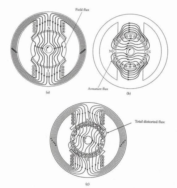
Figure 5.14 (a) Flux distribution due to the field-winding only. (b) Flux distribution due to armature mmf only. (c) Flux distribution due to the field-winding and the armature mmf.
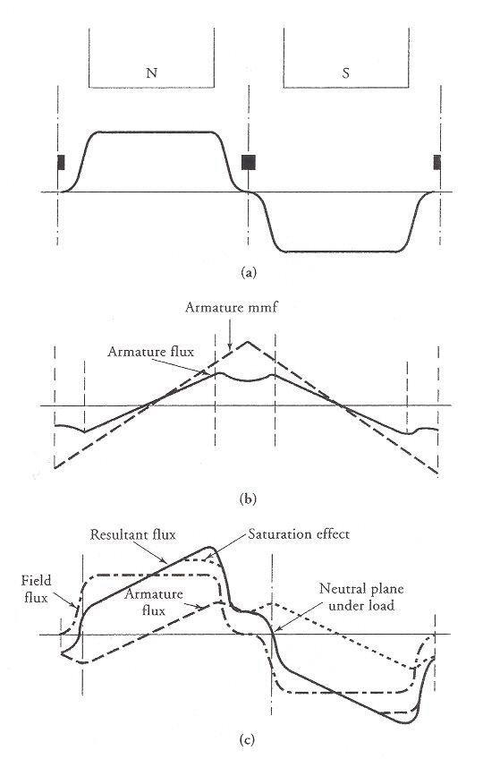
Figure 5.15 (a) Flux per pole under no load. (b) MMF and the flux due to armature reaction. (c) Resultant flux.
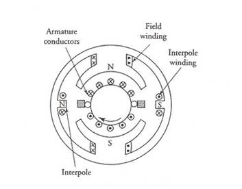
Figure 5.16 Interpole windings of a dc generator.
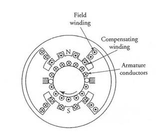
Figure 5.17 Compensating winding of a dc generator.
As the armature flux varies with the load, so does its influence on the flux set up by the field winding. Hence, the shift in the neutral plane is a function of the armature current.
The armature reaction has a demagnetizing effect on the machine. The reduction in the flux due to armature reaction suggests a substantial loss in the applied mmf per pole of the machine. In large machines, the armature reaction may have a devastating effect on the machines performance under full load.
Therefore, techniques must be developed to counteract its demagnetization effect. Some of the measures that are being used to combat armature reaction are summarized below:
The brushes may be advanced from their neutral position at no load (geometrical neutral axis) to the new neutral plane under load. This measure is the least expensive. However, it is useful only for constant-load generators.
Interpoles, or commutating poles as they are sometimes called, are narrow poles that may be located in the interpolar region centered along the mechanical neutral axis of the generator. The interpole windings are permanently connected in series with the armature to make them effective for varying loads. The interpoles produce flux that opposes the flux due to the armature mmf. When the interpole is properly designed, the net flux along the geometric neutral axis can be brought to zero for any load. Because the interpole winding carries armature current, we need only a few turns of comparatively heavy wire to provide the necessary interpole mmf. Figure 5.16 shows the armature flux distribution with interpoles.
Another method to nullify the effect of armature reaction is to make use of compensating windings. These windings, which also carry the armature current, are placed in the shallow slots cut in the pole faces as shown in Figure 5.17. Once again, the flux produced by the compensating winding is made equal and opposite to the flux established by the armature mmf.
5.9 Types of DC Generators
Based upon the method of excitation, dc generators can be divided into two classes Separately excited generators and self-excited generators. A PM generator can be considered a separately excited generator with constant magnetic flux.
The field (excitation) current in a separately excited generator is supplied by an independent external source. However, a self-excited generator provides its own excitation current. According to the method of connection of the field winding(s), a self-excited generator can be further classified as (a) a shunt generator if its field winding, called the shunt field winding, is connected across the armature terminals (b) a series generator when its field winding, called the series field winding, is connected in series with the armature, and (c) a compound generator with both shunt and series field windings.
We investigate the operation of each type of dc generator by examining its external characteristics under steady-state conditions. The external characteristic of a dc generator is the variation of the load voltage (terminal voltage) with load current. This information enables us to highlight the application for which each generator is most suitable.
During our discussion of dc generators we should keep in mind the following facts:
The generator is driven by a prime moves, such as a synchronous motor, at a constant speed.
The induced emf in the armature winding is proportional to the flux in the machine; that is, Ea = Ka Fpwm
The armature terminals are connected to the load.
The armature winding has finite resistance, however small it may be. Therefore, the armature terminal voltage is bound to be lower than the induced emf.
If the generator is not compensated for the armature reaction, there is less overall flux in the machine under load than at no load. Thus, the induced emf is lower under load than at no load. This results in a further decrease of the terminal voltage.
The torque developed by the armature conductors, Td = Ka Fp Ia, is equal and opposite to the torque applied by the prime mover. That is, the torque developed opposes the armature rotation.
The voltage drop between the brushes and the commutator segments is known as the brush-contact drop. If needed and not specifies, it may be assumed to be about 2 V.
If the pertinent information regarding the adverse effect of armature reaction on generator performance is not known, we assume that either the armature reaction is negligible or the generator is appropriately compensated for it.
We commonly use a term called load in electrical machines to signify the load-current. Thus, no load means an open circuit and full load implies the rated load-current at the rated terminal voltage.
5.10 Voltage Regulation
As the load-current increases, the terminal voltage decreases owing to the increase in the voltage drop across the armature-winding resistance as well as the demagnetization effect of the armature reaction. The voltage regulation is a measure of the terminal voltage drop at full load. If VnL is the no-load terminal voltage and VfL is the full-load terminal voltage, the voltage regulation is defined as
 (5.22)
where VR% is the percent voltage regulation. For an ideal (constant-voltage) generator, the voltage regulation should be zero. The voltage regulation is considered positive when the terminal voltage at no load is higher than at full load. A negative voltage regulation indicates that the terminal voltage at full load is higher than that at no load.
5.11 Losses in DC Machines
Once again, we are using the term machine in the discussion of power losses owing to the fact that no distinction need be made between the losses in the dc generator and the motor. The law of conservation of energy dictates that the input power must always be equal to the output power plus the losses in the machine. There are three major categories of losses: mechanical losses, copper losses, and magnetic losses.
Mechanical Losses
Mechanical losses are the result of (a) the friction between the bearings and the shaft, (b) the friction between the brushes and the commutator, and (c) the drag on the armature caused by air enveloping the armature (windage loss).
The bearing-friction loss depends upon the diameter of the shaft at the bearing, the shafts peripheral speed, and the coefficient of friction between the shaft and the bearing. To reduce the coefficient of friction, the bearings are usually lubricated.
The brush-friction loss depends upon the peripheral speed of the commutator, the brush pressure, and the coefficient of friction between the brush and the commutator. The graphite in the brush helps provide lubrication to lessen the coefficient of friction.
The windage loss depends upon the peripheral speed of the armature, the number of slots on its periphery, and its length.
Mechanical losses due to friction and windage Pfw can be determined by rotating the armature of an unexcited machine at its rated speed by coupling it to a calibrated motor. Because there is no power output, the power supplied to the armature is the mechanical loss.
Magnetic Loss
Since the induced emf in the conductors of the armature alternates with a frequency determined by the speed of rotation and the number of poles, a magnetic loss Pm (hysteresis and the eddy-current) exists in the armature.
The hysteresis loss depends upon the frequency of the induced emf, the area of the hysteresis loop, the magnetic flux density, and the volume of the magnetic material. The area of the hysteresis loop is smaller for soft magnetic materials than for hard magnetic materials. This is one of the reasons why soft magnetic materials are used for electrical machines.
Although the armature is built using thin laminations, the eddy currents do appear in each lamination and produce eddy-current loss. The eddy-current loss depends upon the thickness of the lamination, the magnetic flux density, the frequency of the induced emf, and the volume of the magnetic material.
A considerable reduction in the magnetic loss can be obtained by operating the machine in the linear region at a low flux density but at the expense of its size and initial cost.
Rotational Losses
In the analysis of a dc machine, it is a common practice to lump the mechanical loss and the magnetic loss together. The sum of the two losses is called the rotational loss, Pr. That is, Pr = Pfw + Pm.
The rotational loss of a dc machine can be determined by running the machine as a separately excited motor (to be discussed later) under no load.
The armature winding voltage should be so adjusted that the induced emf in the armature winding is equal to its rated value, Ea. If Vt is the terminal voltage and Ra is the armature-winding resistance, then the voltage that must be applied to the armature terminals is
![]() (5.23a)
(5.23a)
for the generator and
![]() (5.23b)
(5.23b)
for the motor.
Apply Va across the armature terminals and adjust the field excitation until the machine rotates at its rated speed. Then measure the armature current. Because the armature current under no load is a small fraction of its rated value and the armature winding resistance is usually very small, we can neglect the power loss in the armature winding. As there is no power output, the power supplied to the motor, VaIa, must be equal to the rotational loss in the machine. By subtracting the mechanical loss, we can determine the magnetic loss in the machine.
Copper Losses
Whenever a current flows in a wire, a copper loss, Pcu, is associated with it. The copper losses, also known as electrical or I2R losses, can be segregated as follows:
Armature-winding loss
Shunt field- winding loss
Series field- winding loss
Interpole field- winding loss
Compensating field- winding loss
Stray-Load Loss
A machine always has some losses that cannot be easily accounted for; they are termed stray-load losses. It is suspected that the stray-load losses in dc machines are the result of (a) the distorted flux due to armature reaction and (b) short-circuit currents in the coils undergoing commutation. As a rule of thumb, the stray-load loss is assumed to be 1% of the power output in large machines (above 100 horse-power) and can be neglected in small machines.
Power-Flow Diagram
In a dc generator, the mechanical energy supplied to the armature by the prime mover is converted into electric energy. At the outset, some of the mechanical energy is lost as the rotational loss. The mechanical power that is available for conversion into electrical power is the difference between the power supplied to the shaft and the rotational loss. We refer to the available power as developed power. Subtract all the copper losses in the machine from the developed power to obtain the power output. If Ts is the torque at the shaft and wm is the angular velocity of rotation, then the power output, P0, for a generator is
![]() (5.24)
(5.24)
A typical power-flow diagram for the generator is shown in Figure 5.18.
Efficiency
The efficiency of a machine is simply the ratio of its power output to the power input. In the case of a separately excited machine, the power lost in the field winding may also be included in the input power when computing the efficiency of the machine.

Figure 5.18 Power-flow diagram of a dc generator.
5.12 A Separately Excited DC Generator
As the name suggests, a separately excited dc generator requires an independent dc external source for the field winding and for this reason is used primarily in (a) laboratory can be another dc generator, a controlled or uncontrolled rectifier, or simply a battery.
The equivalent circuit representation under steady-state condition of a separately excited dc generator is given in Figure 5.19. The steady-state condition implies that no appreciable change occurs in either the armature current or the armature speed for a given load. In other words, there is essentially no change in the mechanical energy or the magnetic energy of the system. Therefore, there is no need to include the inductance of each winding and the inertia of the system as part of the equivalent circuit.
In the equivalent circuit, Ea is the induced emf in the armature winding, Ra is the effective armature-winding resistance which may also include the resistance of each brush, Ia is the armature current, Vt is the terminal output voltage, IL is the load current, If is the field-winding current, Rfw is the field-winding resistance, Rfx is an external resistance added in series with the field winding to control the field current, Nf is the number of turns per pole for the field winding, and Vf is the voltage of an external source.
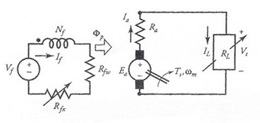
Figure 5.19 An equivalent circuit of a separately excited dc generator.
The defining equations under steady-state operation are
![]() (5.25)
(5.25)
![]() (5.26)
(5.26)
and
![]() (5.26a)
(5.26a)
where Rf = Rfw + Rfx is the total resistance in the shunt field-winding circuit.
From Eq. (5.26), the terminal voltage is
![]() (5.27)
(5.27)
When the field current is held constant and the armature is rotating at a constant speed, the induced emf in an ideal generator is independent of the armature current, as shown by the dotted line in Figure 5.20. As the load current IL increases, the terminal voltage Vt decreases, as indicated by the solid line. In the absence of the armature reaction, the decrease in Vt should be linear and equal to the voltage drop across Ra. However, if the generator is operating near its saturation and is not properly compensated for the armature reaction, the armature reaction causes a further drop in the terminal voltage.
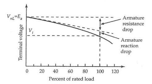
Figure 5.20 The external characteristic of a separately excited dc generator.
A plot of the terminal voltage versus the load current is called the external (terminal) characteristic of a dc generator. The external characteristic can be obtained experimentally by varying the load from no load to as high as 150% of the rated load. The terminal voltage at no load, VnL, is simply Ea. If we draw a line tangent to the curve at no load, we obtain the terminal characteristic of the machine with no armature reaction. The difference between the no-load voltage and the tangent line yields IaRa drop. Since Ia is known, we can experimentally determine the effective armature-winding resistance. The term effective signifies that it is not only the resistance of the armature winding but also includes the brush-contact resistance.
5.13 A Shunt Generator
When the field winding of a separately excited generator is connected across the armature, the dc generator is called the shunt generator. In this case, the terminal voltage is also the field-winding (field) voltage. Under no load, the armature current is equal to the field current. When loaded, the armature current supplies the load current and the field current as shown in Figure 5.21. Since the terminal voltage can be very high, the resistance of the field circuit must also be high in order to keep its power loss to a minimum. Thus, the shunt field winding has a large number of turns of relatively fine wire.
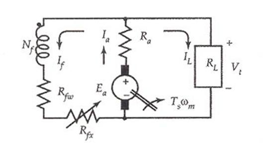
Figure 5.21 An equivalent circuit of a shunt generator.
As long as some residual flux remains in the field poles, the shunt generator is capable of building up the terminal voltage. The process of voltage buildup is summarized below.
When the generator is rotating at its rated speed, the residual flux in the field poles, however small is may be (but is must be there), induces an emf Er in the armature winding as shown in Figure 5.22. Because the field winding is connected across the armature, the induced emf sends a small current through the field winding. If the field winding is properly connected, its mmf sets up a flux that aids the residual flux. The total flux per pole increases. The increase in the flux per pole increases the induced emf which, in turn, increases the field current. The action is therefore cumulative. Does this action continue forever? The answer, of course, is no for the following reason:
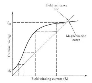
Figure 5.22 Voltage buildup in a shunt generator.
The induced emf follows the nonlinear magnetization curve. The current in the field winding depends upon the total resistance in the field-winding circuit. The relation between the field current and the field voltage is linear, and the slope of the curve is simply the resistance in the field-winding circuit. The straight line is also known as the field-resistance line. The shunt generator continues to build up voltage until the point of intersection of the field-resistance line and the magnetic saturation curve. This voltage is known as the no-load voltage.
It is very important to realize that the saturation of the magnetic material is a blessing in the case of a self-excited generator. Otherwise, the voltage buildup would continue indefinitely. We will also show that the saturation is necessary for the generator to deliver load.
If the field winding is connected in such a way that the flux produced by its mmf opposes the residual flux, a voltage build-down will occur. This problem can be corrected by either reversing the direction of rotation or interchanging the field-winding connection to the armature terminals, but not both.
The value of no-load voltage at the armature terminals depends upon the field-circuit resistance. A decrease in the field-circuit resistance causes the shunt generator to build up faster to a higher voltage as shown in Figure 5.23. By the same token, the voltage buildup slows down and the voltage level falls when the field-circuit resistance is increased. The value of the field-circuit resistance that makes the field-resistance line tangent to the magnetization curve is called the critical (field) resistance. The generator voltage will not build up if the field-circuit resistance is greater than or equal to the critical resistance. The speed at which the field circuit resistance becomes the critical resistance is called the critical speed.
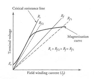
Figure 5.23 Voltage buildup for various values of field-circuit resistances.
Hence, the voltage buildup will take place in a shunt generator if (a) a residual flux exists in the field poles, (b) the field-winding mmf produces the flux that aids the residual flux, and (c) the field-circuit resistance is less than the critical resistance.
The equations that govern the operation of a shunt generator under steady-state are
![]() (5.28)
(5.28)
![]() (5.29)
(5.29)
and
![]() (5.30)
(5.30)
The External Characteristic
Under no load, the armature current is equal to the field current, which is usually a small fraction of the load current. Therefore, the terminal voltage under no-load VnL is nearly equal to the induced emf Ea owing to the negligible IaRa drop. As the load current increases, the terminal voltage decreases for the following reasons:
The increase in IaRa drop
The demagnetization effect of the armature reaction
The decrease in the field current due to the drop in the induced emf
The effect of each of these factors is shown in Figure 5.24.
For a successful operation, the shunt generator must operate in the saturated region. Otherwise, the terminal voltage under load can fall to zero for the following reason:
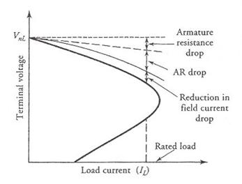
Figure 5.24 External characteristic of a shunt generator.
Suppose the generator is operating in the linear region and there is a 10% drop in the terminal voltage as soon as the load draws some current. A 10% drop in the terminal voltage results in a 10% drop in the field current which, in turn, reduces the flux by 10%. A 10% reduction in the flux decreases the induced emf by 10% and causes the terminal voltage to fall even further, and so on. Soon the terminal voltage falls to a level (almost zero) that is not able to supply any appreciable load. The saturation of the magnetic material comes to the rescue. When the generator is operating in the saturated region, a 10% drop in the field current may result in only a 2% or 3% drop in the flux, and the system stabilizes at a terminal voltage somewhat lower than VnL but at a level suitable for successful operation.
As the generator is loaded, the load current increases to a point called the break-down point with the decrease in the load resistance. Any further decrease in the load resistance results in a decrease in the load current owing to a very rapid drop in the terminal voltage. When the load resistance is decreased all the way to zero (a short circuit), the field current goes to zero and the current through the short circuit is the ratio of the residual voltage and the armature-circuit resistance.
5.14 A Series Generator
As the name suggests, the field winding of a series generator is connected in series with the armature and the external circuit. Because the series field winding has to carry the rated load current, it usually has few turns of heavy wire.
The equivalent circuit of a series generator is given in Figure 5.25. A variable resistance Rd, known as the series field diverter, may be connected in shunt with the series field winding to control the current through and thereby the flux produced by it.
When the generator is operating under no load, the flux produced by the series field winding is zero. Therefore, the terminal voltage of the generator is equal to the induced emf due to the residual flux, Er. As soon as the generator supplies a load current, the mmf of the series field winding produces a flux that aids the residual flux. Therefore, the induced emf, Er, in the armature winding is higher when the generator delivers power than that at no load. However, the terminal voltage, Vt, is lower than the induced emf due to (a) the voltage drops across the armature resistance, Ra, the series field-winding resistance, Rs, and (b) the demagnetization action of the armature reaction. Since voltage drops across the resistances and the armature reaction are functions of the load current, the induced emf and thereby the terminal voltage depend upon the load current.
The magnetization curve for the series generator is obtained by separately exciting the series field winding. The terminal voltage corresponding to each point on the magnetization curve is less by the amount equal to voltage drops across Ra and Rs when the armature reaction is zero. The terminal voltage drops even further when the armature reaction is also present as illustrated in Figure 5.26. Once the load current pushes the generator into the saturated region, any further increase in its value makes the armature reaction so great as to cause the terminal voltage to drop sharply. In fact, if driven to its extreme, the terminal voltage may drop to zero.
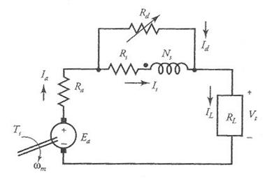
Figure 5.25 An equivalent circuit of a series generator.
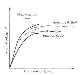
Figure 5.26 Characteristics of a series generator.
The rising characteristic of a
series generator makes it suitable for voltage-boosting purposes. Another clear
distinction between a shunt generator and a series generator is that the shunt
generator tends to maintain a constant
terminal voltage while the series generator has a tendency to supply constant load current. In
The basic equations that govern its steady-state operation are
![]() (5.31)
(5.31)
![]() (5.32)
(5.32)
![]() (5.33)
(5.33)
where Is is the current in the series field winding, Rs is the resistance of the series field winding, and Ld is the current in the series field-diverter resistance, Rd.
5.15 Compound Generators
The drooping characteristic of a shunt generator and the rising characteristic of a series generator provide us enough motivation to theorize the possibility of a better external characteristic by fusing the two generators into one. In fact, under certain constraints, putting the two generators together is like transforming two contentiously different generators into a single well-behaved generator.
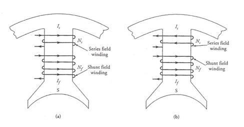
Figure 5.27 Current distributions in the series and the shunt field windings of
(a) cumulative and (b) differential compound generators.
This is done by winding both series and shunt field windings on each pole of the generator. When the mmf of the series field is aiding the mmf of the shunt field, it is referred to as a cumulative compound generator (Figure 5.27a). Otherwise, it is termed a differential compound generator (Figure 5.27b).
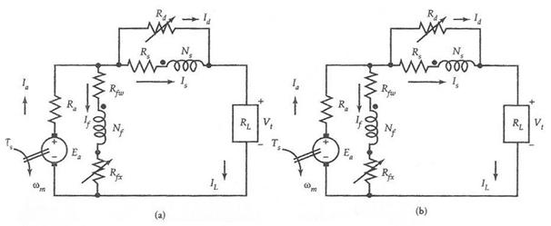
Figure 5.28 Equivalent circuits of short-shunt (a) cumulative and (b) differential compound generators.
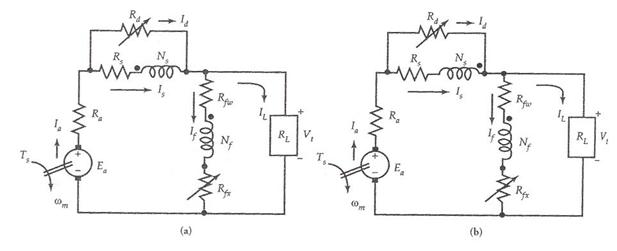
Figure 5.29 Equivalent circuits of long-shunt (a) cumulative and (b) differential compound generators.
When the shunt field winding is connected directly across the armature terminals, it is called a short-shunt generator. In a short-shunt generator (Figure 5.28), the series field winding carries the load current in the absence of a field diverter resistance. A generator is said to be long shunt when the shunt field winding is across the load as indicated in Figure 5.29. We hasten to add that most
of the flux is created by the shunt field. The series field mainly provides a control over the total flux. Therefore, different levels of compounding can be obtained by limiting the current through the series field, as explained in Section 5.14. Three distinct degrees of compounding that are of considerable interest are discussed below.
Undercompound Generator
When the full-load voltage in a compound generator is somewhat higher than that of a shunt generator but still lower than the n-load voltage, it is called an undercompound generator. The voltage regulation is slightly better than that of the shunt generator.
Flat or
When the no-load voltage is equal to the full-load voltage, the generator is known as a flat compound generator. A flat compound generator is used when the distance between the generator and the load is short. In other words, no significant voltage drop occurs on the transmission line (called the feeder) connecting the generator to the load.
Overcompound Generator
When the full-load voltage is higher than the no-load voltage, the generator is said to be overcompound. An overcompound generator is the generator of choice when the generator is connected to a load via a long transmission line. The long transmission line implies a significant drop in voltage and loss in power over the transmission line.
The usual practice is to design an overcompound generator. The adjustments can then be made by channeling the current away from the series field winding by using the field diverter resistance.
The external characteristics of compound generators are given in Figure 5.30. For comparison purposes, the external characteristics of other generators are also included.
The fundamental equations that govern the steady-state behavior of short-shunt and long-shunt cumulative generators are given below.
Short-shunt:
![]() (5.34)
(5.34)
 (5.35)
![]() (5.36)
(5.36)
![]() (5.37)
(5.37)
![]() (5.38)
(5.38)
where the (plus/minus) sign is for the (cumulative/differential) compound generator, and mmfd is the demagnetizing mmf due to the armature reaction.
Long-shunt:
![]() (5.39)
(5.39)
 (5.40)
![]() (5.41)
(5.41)
![]() (5.42)
(5.42)
5.16 Maximum Efficiency Criterion
Either by performing an actual load test on a given machine or just by calculating its performance at various loads, we can obtain an efficiency versus load curve. It would become evident from this curve that the efficiency increases with load up to some point where it becomes maximum. Any increase in the load thereafter causes a decrease in efficiency. It is, therefore, imperative to know at what load the efficiency of the machine is maximum. Operating the machine at its maximum efficiency results in (a) a decrease in the losses in the machine, which, in turn, drops the operating temperature of the machine, and (b) a reduction in the operating cost of the machine.
Prior to deriving an expression that determines the load at which a generator provides maximum efficiency, let us first take another look at the losses. The losses in a generator can be grouped in two categories: fixed losses and variable losses. Fixed losses do not vary with the load when the generator is driven at a constant speed. The rotational loss falls into this category. Although it is not strictly true for self-excited generators, the shunt-field current, If. Is taken to be constant. Thus, the power loss due to If can also be considered a part of the fixed loss. The variable loss, on the other hand, is the loss that varies with the load current.
For a PM dc generator, the power output is
![]()
and the power input is
![]()
Hence, the efficiency is
For the efficiency to be maximum, the rate of change of h with respect to IL must be zero when IL Ilm, where Ilm is the load current at maximum efficiency. That is
From this we obtain
![]() (5.43)
(5.43)
Hence, the load current at maximum efficiency for a PM dc generator is
 (5.44)
The conditions for the maximum efficiency for other generators are as follows:
Separately excited:
![]() (5.45)
(5.45)
Shunt:
![]() (5.46)
(5.46)
Series:
![]() (5.47)
(5.47)
Short-shunt:
![]() (5.48)
(5.48)
Long-shunt:
![]() (5.49)
(5.49)
SUMMARY
We devoted this chapter entirely to the study of different types of dc generators. Most of the principles we have introduced in this chapter are equally applicable to dc machines. The main components of a dc machine are the stator, the armature, and the commutator.
The induced emf in the armature winding varies sinusoidally with a frequency of
However, the commutator rectifies it and we get almost constant voltage output. The dc-generated voltage is
![]()
and the torque developed by the generator is
![]()
The prime mover must apply the torque in a direction opposite to the torque developed. The applied mechanical energy is then converted into electrical energy.
The armature is either lap wound or wave wound using a two-layer winding. In a lap winding, the two ends of the coil are connected to the adjacent commutator segments. The two ends are almost 360o electrical apart in the case of a wave winding. The lap winding offers as many parallel paths as there are poles in the machine. There are only two parallel paths in a wave-wound machine.
In order to predict the performance of a machine, we need information on its magnetic saturation. This information is usually presented in the form of a magnetization curve. For successful operation of a self-excited generator, the point of operation must be in the saturation region.
The current in the armature winding produces its own flux, which has a demagnetizing effect, called armature reaction, on the machine. Techniques such as interpoles and/or commutating windings are used to minimize the armature reaction. When the machine operates at a constant load, advancing the brushes from their geometric neutral axis to the new neutral axis may do the trick.
There are two basic types of generators: separately excited and self-excited. Self-excited generators are further classified as shunt, series, and compound. Except for the overcompound generator, the terminal voltage of all other generators falls as a function of the load current. The voltage regulation is simply a measure of the change in the terminal voltage at full load.
The losses in a dc machine reduce its efficiency. We have categorized the losses as the rotational loss, the copper loss, and the stray-load loss. The rotational loss accounts for the mechanical power loss due to friction and windage, and the magnetic power loss is due to eddy currents and hysteresis. The copper loss accounts for all the electrical losses in the machine. When a loss cannot be properly accounted for, it is considered as a part of the stray-load loss.
|
Politica de confidentialitate | Termeni si conditii de utilizare |

Vizualizari: 5815
Importanta: ![]()
Termeni si conditii de utilizare | Contact
© SCRIGROUP 2025 . All rights reserved