| CATEGORII DOCUMENTE |
| Bulgara | Ceha slovaca | Croata | Engleza | Estona | Finlandeza | Franceza |
| Germana | Italiana | Letona | Lituaniana | Maghiara | Olandeza | Poloneza |
| Sarba | Slovena | Spaniola | Suedeza | Turca | Ucraineana |
In this lecture the fundamental definitions and concepts used in the Mechanics of Materials are presented.
Static Equilibrium of Deformable Solid Body
In this textbook only the time independent loads, the static loads, are considered to act on the three-dimensional solid. Consequently, the inertial forces are zero and the necessary conditions for equilibrium are expressed as:
![]() (1)
(1)
![]() (2)
(2)
where the notation stands for:
![]() - is the number of
concentrated forces;
- is the number of
concentrated forces;
![]() - is the force resultant
vector and its components;
- is the force resultant
vector and its components;
![]() are the magnitude of
the components of
are the magnitude of
the components of![]() along the coordinate axes;
along the coordinate axes;
![]() - is a particular
force;
- is a particular
force;
![]() - are the magnitude of
the components of
- are the magnitude of
the components of![]() along the coordinate axes;
along the coordinate axes;
![]() - are the Cartesian
unit vectors of the
- are the Cartesian
unit vectors of the ![]() system;
system;
![]() - is the moment resultant
vector and its components calculated at the arbitrary point
- is the moment resultant
vector and its components calculated at the arbitrary point![]() , the origin of the
, the origin of the ![]() coordinate system;
coordinate system;
![]() - are the magnitude of
the components of
- are the magnitude of
the components of ![]() along the coordinate axes;
along the coordinate axes;
![]() - is the position
vector extending from the coordinate origin to the point where the concentrated
force
- is the position
vector extending from the coordinate origin to the point where the concentrated
force ![]() is applied.
is applied.
The vectorial equations (1) and (2) can be re-written in a scalar form of six algebraic equations:
![]() (3)
(3)
![]() (4)
(4)
![]() (5)
(5)
![]() (6)
(6)
![]() (7)
(7)
![]() (8)
(8)
The equations of equilibrium (3) through (8) were previously developed and extensively used in the Classical Mechanics course, where the three-dimensional rigid solid was studied.
The mathematical statements, (1) and (2), imply that the three-dimensional solid body is free of constraints, a situation contradictory to the norm where the constraints are present. It should be noted that the equilibrium equations do not refer in any way to the nature of the material present in the solid or to any type of deformation. Consequently, those equations also apply fully in the general case of a deformable three-dimensional solid.
To utilize the equations (1) and (2) under the usual conditions, the three-dimensional deformable solid is released from its constraints, and these are replaced with the corresponding reaction forces. As described in section 1.3, the drawing that illustrates the geometry of the three-dimensional solid, the exterior actions, and the unknown reaction forces is called a free-body diagram. A generic example of a free-body diagram is shown in Figure 1.
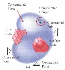
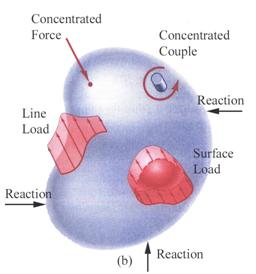
Figure 1 Generic Free-Body Diagrams
(a) Constrained Body, (b) Free Body
The attempt to write the equations of equilibrium, (3) through (8), using the active forces and the reaction forces, results in a system of six algebraic equations with constant coefficients, containing the reaction forces as unknown quantities. This system of equations may be solved using any linear algebra method of solution for algebraic equation systems with constant coefficients. If the equations contain only six unknown reactions it is called a statically determinate system and, consequently, can be solved. When the number of unknown reactions is higher than six, the equation system is called a statically indeterminate system and additional equations are required for the reactions to be calculated. If a number of supports can be removed without destroying the static equilibrium of the body, those supports may be identified as redundant supports and the corresponding reaction forces are called redundants.
In the particular case of the
plane linear beam when the exterior acting loads and the reaction forces are
contained in the vertical plane ![]() only three equations
of equilibrium from the initial six are required for solution as follows:
only three equations
of equilibrium from the initial six are required for solution as follows:
![]() (9)
(9)
![]() (10)
(10)
![]() (11)
(11)
Note: It can be shown that only the number of equilibrium equation is fixed at six, but the option of writing these equations vary. For the plane case the equations (9) through (11) may be replaced, for example, by one force equation and two moment equations.
Support Reaction Forces and Beam Connections
The external loads applied on the
three-dimensional deformable body are carried to the supports, which are the points where the interaction with the
environment (other bodies) is considered to take place. At the supporting
points the displacements, represented by a change in the position of the point,
are known quantities with prescribed value. In general, the supported point is
constrained against movement in some direction and thus, the displacement in
that direction is zero. There are also cases where a displacement of known
magnitude and/or direction is imposed a particular support point. Due to the
If the studied system is composed of more than one single body, the common points between each adjoining body are called connections. To write the equilibrium equations for a multi- body system the connections should also be replaced by reaction forces. A free-body diagram and a set of equilibrium equations may then be constructed for each body allowing for solution of all external support reaction as well as for all internal connection reactions.
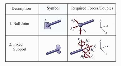
Tables 1 through 3 contain the most common idealized types of supports and their corresponding reaction forces. The two-dimensional cases are illustrated in Tables 1 and 2 which are directly related with the behavior of the linear plane beam, the case of interest for this course. The supports and reactions pertinent to the three-dimensional case, only occasionally considered in this course, are depicted in Table 3 for completeness.
Table 1 Plane Supports and Reactions
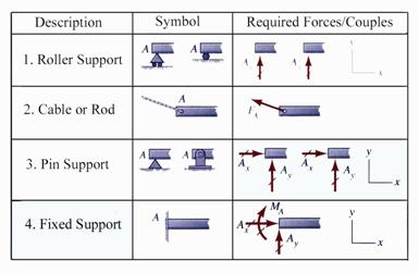
Table 2 Plane Connections and Reactions
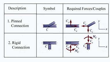
Table 3 Three-Dimensional Supports and Reactions
Generalized Stress Tensor and Components
When subjected to external actions, the three-dimensional solid deforms and the internal original equilibrium is disturbed. To determine the internal forces located in the volume of the deformed body the method of sections is employed. The application of the methodology is depicted in Figures 2 and 3.
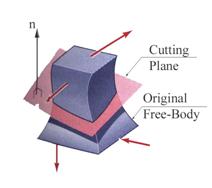
Figure 2 Three-Dimensional Free-Body Sectioned by a Cutting Plane
Practically, the original body is divided into two parts, each one carrying its portion of exterior and reaction forces, by an arbitrarily orientated plane. In a manner of speaking, the cutting plane plays, the role of the member connection. As in the connection case, the broken continuity of the body is replaced by internal forces acting at every point of the common surface.
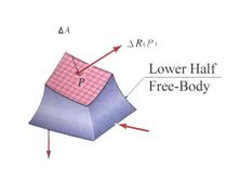
Figure 3 Lower Half of the Sectioned Original Body
The internal force![]() is called the stress
vector or traction and acts on
the elementary surface
is called the stress
vector or traction and acts on
the elementary surface![]() located in the vicinity of point
located in the vicinity of point ![]() (see Figure 3). Using
a local coordinate system
(see Figure 3). Using
a local coordinate system ![]() attached to the
current point
attached to the
current point![]() , where
, where ![]() represents the unit
vector normal to the cutting plane, the stress vector
represents the unit
vector normal to the cutting plane, the stress vector ![]() is decomposed into three components,
is decomposed into three components,![]() ,
, ![]() and
and ![]() . The decomposition process is illustrated in Figure 4. The
first component of the stress vector,
. The decomposition process is illustrated in Figure 4. The
first component of the stress vector,![]() , is orientated parallel to the surface outside normal unit
vector
, is orientated parallel to the surface outside normal unit
vector![]() , while the other two components,
, while the other two components, ![]() and
and![]() , are located in the cutting plane.
, are located in the cutting plane.
Note: The normal ![]() is univocally defined by the choice of cutting plane, while
the other two directions,
is univocally defined by the choice of cutting plane, while
the other two directions, ![]() and
and ![]() are arbitrarily chosen under the condition that the three are
mutually perpendicular.
are arbitrarily chosen under the condition that the three are
mutually perpendicular.
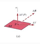
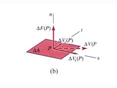
Figure 4 Stress Vector and Components
The components of the stress tensor located in a three-dimensional solid body are defined through a limiting process.
The position
of the point ![]() is uniquely defined by
its position vector
is uniquely defined by
its position vector![]() . The stress tensor
. The stress tensor![]() is called normal
stress and acts normal to the cutting plane. The in-plane stress tensors
is called normal
stress and acts normal to the cutting plane. The in-plane stress tensors![]() and
and ![]() are called shear
stresses.
are called shear
stresses.
Note: The normal and shear stresses belong to a special mathematical category of algebra named tensors. It is beyond the scope of this course to elaborate on the mathematical properties of tensors, but it must be emphasized that they may not be manipulated as vectors. The stress tensor is transformed into a corresponding stress vector through multiplication with an area and, only then, manipulated through the familiar vectorial algebra.
Some
clarifications regarding the sign convention of the stress tensors are
necessary. The subscript ![]() indicates that the
stresses are pertinent to the surface which has the outward normal vector
indicates that the
stresses are pertinent to the surface which has the outward normal vector ![]() . It is understood that the normal stress
. It is understood that the normal stress![]() is positive when parallel to
is positive when parallel to ![]() , while the in-plane shear stresses
, while the in-plane shear stresses ![]() and
and ![]() are positive when they
are parallel to the
are positive when they
are parallel to the ![]() and
and ![]() axes, respectively.
axes, respectively.
If a new stress
vector ![]() pertinent to the
surface characterized by the outward normal
pertinent to the
surface characterized by the outward normal ![]() is defined the
following vectorial equation can be written:
is defined the
following vectorial equation can be written:
![]() (15)
(15)
After the
algebraic simplification the fundamental relation between the surface stress tensor
![]() and the normal and
shear tensors can be expressed as:
and the normal and
shear tensors can be expressed as:
![]() (16)
(16)
If a set of
three mutually orthogonal planes, defined by a Cartesian general system and
passing through the arbitrarily chosen point ![]() are used, as shown in Figure 5, then three corresponding sets
of stress tensors are obtained by successively considering the unit vectors
are used, as shown in Figure 5, then three corresponding sets
of stress tensors are obtained by successively considering the unit vectors![]() ,
, ![]() and
and ![]() as the normal vector
of the cutting plane.
as the normal vector
of the cutting plane.
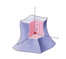
Figure 5 Set of Three Mutually Orthogonal Planes
Consequently, the equation (16) is written for each one of the three orthogonal planes as follows:
![]() (17)
(17)
![]() (18)
(18)
![]() (19)
(19)
The resulting stress tensors are depicted in Figure 6.
The following close examination and discussion of the orientation of the three sets of tensors shown in Figure 6 defines the sign convention used.
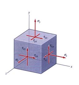
Figure 6 Three-Dimensional Stress Tensors (Cartesian Axes)
The normal stresses are positive when orientated parallel to the outward normal of the surface. They tend to pull the plane and consequently are said to be positive in tension. The shear stress tensor is considered to be positive when orientated parallel to and in the positive direction of the corresponding in-plane axis. These shear stress tensors are identified by two subscripts: the first subscript indicates the plane on which the shear stress acts by the axis defining its normal; the second subscript indicates the shear stress direction by identifying the coordinate system axis to which the shear tensor is aligned.
In Figure 6, for clarity reasons, only the stress tensors pertinent to the visible faces are shown. For the parallel planes having negative axes as normal the stresses have opposite signs. Why? The infinitesimal volume has to be in equilibrium.
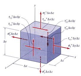
Figure 7 Three-Dimensional Free-Body Diagram of an Infinitesimal Volume
Employing the notation convention described above, it is observed that the shear stress tensors converging towards any particular edge have the subscript order reversed. Consider the situation depicted in Figure 7, where for clarity only the stress tensors which can be used in writing a moment equation around the oz axis are retained.
Note: The Figure 7 is simply a free-body diagram for an elementary volume located around a point P.
The sign
convention previously explained is used. The usage of the superscript ![]() or (-) indicates the variation
of the same stress tensor in-between two parallel faces. The following equations
relating identical stress tensors located on parallel faces, where the position
vector
or (-) indicates the variation
of the same stress tensor in-between two parallel faces. The following equations
relating identical stress tensors located on parallel faces, where the position
vector ![]() has been drop in the notation, are written as:
has been drop in the notation, are written as:
![]() (20)
(20)
![]() (21)
(21)
![]() (22)
(22)
![]() (23)
(23)
![]() (24)
(24)
![]() (25)
(25)
Note: The variation of the stresses between the parallel faces is due to the existence of the exterior actions.
For the infinitesimal volume to be in equilibrium the total moment induced by the stress vectors must be zero.
![]() (26)
(26)
![]() (27)
(27)
![]() (28)
(28)
The moment
component ![]() written about the
written about the ![]() axis considering the
right-hand rule is expressed as:
axis considering the
right-hand rule is expressed as:
 (29)
(29)
Substituting the relations (20) through (25) and (29) into the equilibrium equation (28), equation (30) is obtained:
![]() (30)
(30)
Note: The final expression of the equation (30) is
obtained by neglecting the product of the change in stress (![]() or
or![]() ) and the geometrical elementary quantities (
) and the geometrical elementary quantities (![]() ,
,![]() and
and![]() ) as being very small quantity as
) as being very small quantity as![]() ,
,![]() and
and ![]() tends to zero.
tends to zero.
The equation (30) indicates that for the equilibrium to be enforced, the edge converging shear stress tensors are equal. The equality of the edge converging shear tensors is called the duality principle of the shear stress tensors and is expressed as:
![]() (31)
(31)
It can be concluded that even in the presence of the normal stresses the shear stresses must satisfy the equation (31)
In a similarly
manner, the other two equilibrium equations (26) and (27) involving moments around
![]() and
and ![]() axes are written and the duality of the other shear stresses
is obtained:
axes are written and the duality of the other shear stresses
is obtained:
![]() (32)
(32)
![]() (33)
(33)
The stress tensors can be collected in a tabular form called the generalized stress tensor:
 (34)
(34)
The generalized
stress tensor![]() , which plays an important role in the deformable solid theory,
has nine stress tensors components, but due to the duality principle only six
are independent.
, which plays an important role in the deformable solid theory,
has nine stress tensors components, but due to the duality principle only six
are independent.
Note: It has to be emphasized
that the general stress tensor ![]() is point dependent.
is point dependent.
Saint Venants Principle
The Saint Venants Principle is not a rigorous law of Mechanics of Materials, but has a great practical significance in the analysis of beams and other deformable bodies.
The theoretical explanation of the Saint Venants Principle is depicted in the Figure 8.
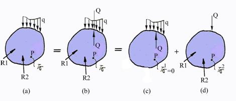
Figure 8 Saint Venants Principle
The original
free-body diagram of the three-dimensional body in equilibrium is shown in
Figure 8.a. The three-dimensional solid is loaded with a force![]() distributed over a small surface of area
distributed over a small surface of area![]() . Suppose that the generalized stress tensor
. Suppose that the generalized stress tensor ![]() is known for any
current point
is known for any
current point![]() of the solid body, identified by its position vector
of the solid body, identified by its position vector![]() . Two concentrated loads of magnitude
. Two concentrated loads of magnitude ![]() opposing each other and acting collinearly with the resultant
of the distributed force
opposing each other and acting collinearly with the resultant
of the distributed force ![]() are superimposed on
the three-dimensional body as shown in Figure 8.b. Their magnitude
are superimposed on
the three-dimensional body as shown in Figure 8.b. Their magnitude ![]() is obtained by integrating the variation of the distributed
force
is obtained by integrating the variation of the distributed
force ![]() over area
over area![]() :
:
![]() (35)
(35)
Proceeding in
this manner, the equilibrium of the three-dimensional solid body remained
unchanged and consequently, the generalized stress tensor![]() remains unaffected. The new loading situation shown in Figure
28.b may then be divided into two load cases as indicated in Figures 8.c and 8.d.
The original generalized tensor
remains unaffected. The new loading situation shown in Figure
28.b may then be divided into two load cases as indicated in Figures 8.c and 8.d.
The original generalized tensor ![]() is written as the sum of
two new generalized stress tensors
is written as the sum of
two new generalized stress tensors ![]() and
and![]() , each one corresponding to the loading situation illustrated
in Figure 8.c and 8.d, respectively.
, each one corresponding to the loading situation illustrated
in Figure 8.c and 8.d, respectively.
![]() (36)
(36)
Note: This relation is valid only under the restrictions of the Principle of Linear Superposition discussed in section 8.
Because the
loads shown in Figure 8.c are self-equilibrated (force and moment resultants
are zero) the generalized stress tensor ![]() calculated in points away
from the loading is expected to tend toward a zero value.
calculated in points away
from the loading is expected to tend toward a zero value.
![]() (37)
(37)
Consequently, the
original generalized tensor ![]() is approximated by the generalized stress tensor
is approximated by the generalized stress tensor![]() pertinent to the loading situation contained in Figure 28.d:
pertinent to the loading situation contained in Figure 28.d:
![]() (38)
(38)
Equation (34) provides validation for Saint Venants Principle.
Beam Stresses and Cross-Section Resultants
The geometrical description of the linear member or beam was given in Section 1.3. Here, it is re-emphasized that the length of the member is much larger than the other two dimensions. Of principal importance in characterizing the behavior of the beam is a geometrical description of its cross-section. The geometrical properties of the cross-section and its theoretical role in the development of the beam theory will be elaborated on during the entire length of these lectures.
Consider the
case of a beam with a general, undefined, geometrical cross-section as shown in
Figure 9. The volume of the beam was sectioned by a normal cutting plane with
its outward normal parallel to the longitudinal local axis ![]() . The general
coordinate system
. The general
coordinate system![]() , previously used, is identical now with the local coordinate
system
, previously used, is identical now with the local coordinate
system ![]() attached to the beam.
attached to the beam.
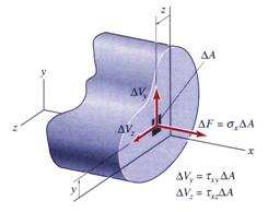
Figure 9 Cross-Section Beam Stresses
In this section the general formulas, expressed in equations (12) through (14), will be applied to the case in point of this textbook, the linear beam.
The normal
stress ![]() is renamed as
is renamed as ![]() , while the shear stresses
, while the shear stresses ![]() and
and ![]() became
became ![]() and
and![]() . The local position vector is written as:
. The local position vector is written as:
![]() (39)
(39)
where ![]() ,
, ![]() and
and![]() are the unit vectors of the local Cartesian coordinate
system.
are the unit vectors of the local Cartesian coordinate
system.
The stress tensor
components ![]() ,
, ![]() and
and![]() can be recomposed in the corresponding stress vectors
can be recomposed in the corresponding stress vectors![]() ,
,![]() , and
, and ![]() , respectively, by multiplying them with the elementary
surface
, respectively, by multiplying them with the elementary
surface ![]() . By integrating over the entire surface of the cross-section
the components of the resultant force and moment particular to the
cross-section are obtained. They are named
cross-sectional resultants and are expressed as:
. By integrating over the entire surface of the cross-section
the components of the resultant force and moment particular to the
cross-section are obtained. They are named
cross-sectional resultants and are expressed as:
![]() (40)
(40)
![]() (41)
(41)
![]() (42)
(42)
![]() (43)
(43)
![]() (44)
(44)
![]() (45)
(45)
The cross-section resultants are depicted in Figure 10.
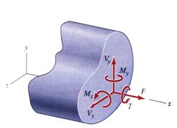
Fig 10 Cross-Sectional Resultants
The
cross-section forces expressed in the equations (40) through (42) are called force resultants. Force ![]() is named cross-section normal force or cross-section axial force, while forces
is named cross-section normal force or cross-section axial force, while forces
![]() and
and ![]() are called cross-section
shear forces. The cross-section normal force is positive if orientated
parallel to the outward normal of the cross-section, while the cross-section
shear forces are positive when orientated parallel to the
are called cross-section
shear forces. The cross-section normal force is positive if orientated
parallel to the outward normal of the cross-section, while the cross-section
shear forces are positive when orientated parallel to the ![]() and
and ![]() positive axes. The
normal force is called the tension
or compression force if the action is in the positive or negative direction of the
cross-section normal, respectively.
positive axes. The
normal force is called the tension
or compression force if the action is in the positive or negative direction of the
cross-section normal, respectively.
The equations
(43) through (45) are written considering that the local coordinate system
follows a right-hand rule and they are called the moment resultants. The moment vector ![]() parallel to
parallel to ![]() axis is named
cross-sectional torsion moment or torque. It has a twisting action on the
cross-section. The other two cross-sectional moments,
axis is named
cross-sectional torsion moment or torque. It has a twisting action on the
cross-section. The other two cross-sectional moments, ![]() and
and ![]() , acting parallel with
, acting parallel with ![]() and
and ![]() positive axes are named
cross-sectional bending moments.
positive axes are named
cross-sectional bending moments.
Extensional and Shear Strains
When subjected
to exterior actions the deformable solid body exhibits volume and shape changes.
Geometrically speaking, this means that the geometry of the body before the
action starts differs from the final geometry. During the deformation process
all of the geometrical characteristics (line segments, angles, surface and
volume) of the solid body are altered. A particular point![]() moves at the end of the deformation process to a new position
moves at the end of the deformation process to a new position![]() . Similarly, the point
. Similarly, the point![]() , located in the vicinity of point
, located in the vicinity of point![]() , is relocated in the new position
, is relocated in the new position![]() . The initial undeformed and final deformed conditions of the
three-dimensional solid body are depicted in Figures 11.a and 11.b, respectively.
. The initial undeformed and final deformed conditions of the
three-dimensional solid body are depicted in Figures 11.a and 11.b, respectively.
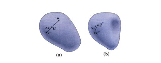
Figure 11 Deformation of the Infinitesimal Line Segment
(a) Undeformed Body and (b) Deformed Body
The infinitesimal
arc![]() , which has arclength
, which has arclength ![]() , is deformed into a new infinitesimal arc
, is deformed into a new infinitesimal arc ![]() with arclength
with arclength ![]() . The definition of
the extensional strain is given
below.
. The definition of
the extensional strain is given
below.
The modification of the original right angle defined by the intersection of two line segments as a result of the deformation process is called shear strain and is schematically shown in Figure 1
Figure 12 Modification of the Right Angle
(a) Undeformed Body and (b) Deformed Body
The original right
angle ![]() changes after the deformation into a new angle
changes after the deformation into a new angle![]() .
.
Definition
2.6 The
shear strain at point
![]() , identified by its
position vector
, identified by its
position vector ![]() , represents the
change of the right angle between
two line segments attached to the point and orientated in directions
, represents the
change of the right angle between
two line segments attached to the point and orientated in directions ![]() and
and![]() , is defined as:
, is defined as: (2.47)
The extensional
and shear strain definitions are generalized for three mutually orthogonal
planes in a similar manner to the development given for the generalized stress
tensor in Section 3. By choosing the Cartesian unit vectors successively as
normal to the cutting planes, the generalized
strain tensor ![]() is obtained:
is obtained:
 (48)
(48)
where:
![]() ),
), ![]() and
and ![]() are the elongation strain measured in the
are the elongation strain measured in the ![]() ,
, ![]() and
and ![]() , respectively;
, respectively;
![]() ,
, ![]() and
and ![]() - are the shear
strains.
- are the shear
strains.
Situations
involving specific the use of specific components of the generalized strain
tensor ![]() are commonly encountered and thus, the subject will be
revisited in the following lectures.
are commonly encountered and thus, the subject will be
revisited in the following lectures.
The rational used in the development of the Saint Venants principal considered only the generalized stress tensor, but a similar argument can be made for the case of the generalized strain tensor.
Constitutive Properties of Materials
The functional expressions relating the generalized stress tensor components to the generalized strain tensor components are called constitutive equations. They reflect the nature of the material contained in the deformable body. Mathematically, a general expression such as equation (45) may be written to define the aforementioned functional relationship:
![]() (49)
(49)
where ![]() - is the component of the generalized stress tensor;
- is the component of the generalized stress tensor;
![]() - is the component of
the generalized strain tensor;
- is the component of
the generalized strain tensor;
![]() - is a given function;
- is a given function;
![]() - is the time
derivative
- is the time
derivative
The functions ![]() are chosen such that
they satisfy the Laws of Thermodynamics and with parameters established by
laboratory testing to give reliable results in physical usage. The change in
the subscripts, from
are chosen such that
they satisfy the Laws of Thermodynamics and with parameters established by
laboratory testing to give reliable results in physical usage. The change in
the subscripts, from ![]() and
and![]() to
to ![]() and
and ![]() , indicates that in general a stress tensor component may be a
function of all the strain tensor components. Only in a few simple cases does a
one-to-one relation exist.
, indicates that in general a stress tensor component may be a
function of all the strain tensor components. Only in a few simple cases does a
one-to-one relation exist.
7.1 Tension Tests
In a laboratory control environment, using a hydraulically actuated testing machine, a material specimen is subjected to a tension test. The schematics of the theoretical tension test are shown in Figure 13.
The tension test
is conducted in the following steps: (a) the original (undeformed) gage length ![]() and cross-sectional
area
and cross-sectional
area ![]() of the specimen are
measured before the test; (b) the ends of the specimen shown in Figure 13.a are
gripped in the testing machine; (c) force is slowly applied to the ends of the
specimen until the rupture of the material is obtained; (d) during the load
application measurements of the gage length
of the specimen are
measured before the test; (b) the ends of the specimen shown in Figure 13.a are
gripped in the testing machine; (c) force is slowly applied to the ends of the
specimen until the rupture of the material is obtained; (d) during the load
application measurements of the gage length ![]() , cross-sectional area
, cross-sectional area ![]() and the value of the
applied forced
and the value of the
applied forced ![]() are tabulated. The
steps (c) and (d) are repeated at regular time intervals and the loading of the
specimen is conducting slowly in order to avoid the rise in temperature and
dynamic effects. When the rupture of the specimen occurs the area
are tabulated. The
steps (c) and (d) are repeated at regular time intervals and the loading of the
specimen is conducting slowly in order to avoid the rise in temperature and
dynamic effects. When the rupture of the specimen occurs the area ![]() is measured once again. This kind of laboratory experiments
will be carried out in the Department Laboratory during the course.
is measured once again. This kind of laboratory experiments
will be carried out in the Department Laboratory during the course.
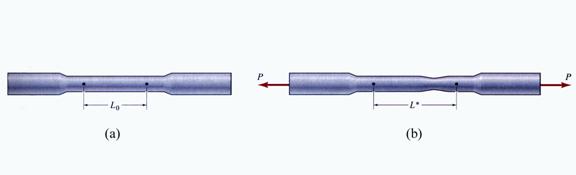
Figure 13 Tension Test of Structural Steel Specimen
(a) Undeformed Specimen, (b) Deformed Specimen
Figure 14 shows the test results obtained from the testing of a structural steel specimen, characterized by low carbon content. To emphasize the test results obtained at lower strain values the beginning end of the test was plotted at a magnified scale. This type of steel is commonly used in structural applications (buildings, bridges, etc.).

Figure 14 Stress-Strain Diagram
The values of the normal stress and elongation strain can be calculated for each loading step as follows:
![]() (50)
(50)
![]() (51)
(51)
where (*) indicates a particular measurement.
The normal stress
defined by the equation (50) is called engineering
stress, while the extension strain expressed by equation (51) is known as
the engineering strain. If the normal
stress is calculated using the value of the step measured area ![]() , the value obtained is called the true stress and the
corresponding strain is called the true
strain. They are calculated as follows:
, the value obtained is called the true stress and the
corresponding strain is called the true
strain. They are calculated as follows:
![]() (52)
(52)
![]() (53)
(53)
Note: The definition (53) is based on the fact that
the volume remained unchanged![]() .
.
The engineering strain and the true strain can are related as expressed by equation (54).
![]() (54)
(54)
Note: Analyzing the expressions of the engineering and true stress and strain it has to be noted that the true values are larger than the engineering values.
7.2 Mechanical Properties of Materials
Several important material properties are obtained from the analysis of the stress-strain diagram. The theoretical behavior of a typical structural steel is illustrated by the stress-strain diagram shown in Figure 15.
The loading and
deformation process begins at point A and continues until point B is reached.
This is the elastic region and is
characterized by a proportionality of the ratio between stress and strain. The point B is named proportional limit occurring when the
stress reaches ![]() . The ratio of stress to strain in the linear range (elastic
region shown) is called the modulus of
elasticity or Youngs modulus and
is designated by the letter
. The ratio of stress to strain in the linear range (elastic
region shown) is called the modulus of
elasticity or Youngs modulus and
is designated by the letter![]() .
.
![]() when
when ![]() (55)
(55)
The units for the modulus of elasticity are stress units (F/L2). Typical units are ksi or GPa.
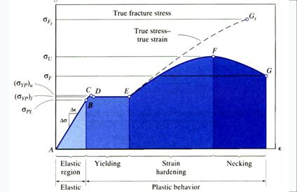
Figure 15 Theoretical Description of the Stress-Strain Diagram
Continuing beyond
the stress and strain characterizing the proportional limit at point B, the
specimen begins to yield. Smaller
incremental loading steps are necessary to induce additional elongation. Two
new points, C and D, named the upper
yielding point,![]() , and the lower
yielding point,
, and the lower
yielding point, ![]() , are obtained. For practical purposes only the lower
yielding point D is retained and will be called the yielding point
, are obtained. For practical purposes only the lower
yielding point D is retained and will be called the yielding point![]() . From point D to point E increased elongation of the
specimen occurs with no increase in stress and consequently, the stress at
point E has an identical value with the stress at point D. As shown in Figure 15,
the diagram is horizontal and the region is called the perfectly plastic region.
. From point D to point E increased elongation of the
specimen occurs with no increase in stress and consequently, the stress at
point E has an identical value with the stress at point D. As shown in Figure 15,
the diagram is horizontal and the region is called the perfectly plastic region.
The stress begins again to increase with increased in elongation after passing point E. The increase continues until point F, where the ultimate stress or the ultimate strength, is reached. The phenomenon and the zone are called strain hardening and strain hardening region, respectively.
If the elongation
of the specimen continues a decrease in the stress is recorded and the
so-called necking appears. The necking represents the visual reduction of
the cross-section and continues until the fracture of the specimen is attended
at point G. The stress calculated at point F, is the maximum stress
characterizing the entire stress-strain diagram. This value is called the ultimate
stress or ultimate strength and
is designated by ![]() .
.
If the material
stress and strain remain in the elastic region where the stress is proportional
the strain, the material exhibits elastic
behavior. If the material is loaded over the proportionality limit ![]() the material exhibits plastic behavior.
the material exhibits plastic behavior.
The material behavior described above is based on the engineering characterization of the stress and strain. For comparison the true stress and strain behavior is also plotted in Figure 15. The true stress-strain diagram is plotted using a dashed line, while the engineering stress-strain diagram is plotted with a heavy continuous line.
The area contained under the stress-strain diagram represents the energy necessary to deform the specimen. It can be noted, from Figures 14 and 15, that the energy characterizing the elastic deformation is considerable smaller than the energy characterizing the plastic deformation. This is an important characteristic typical of ductile materials.
The behavior of the structural steel, as it was described above, can be explained without going into the theoretical details by behavior of the metal micro-structure. Obviously, different metals exhibit different type of stress-strain behavior when subjected to a tension test. To emphasize this observation, the stress-strain diagrams for low carbon steel, three high-strength alloy steels and three aluminum alloys are presented in Figures 16.a and 16.b, respectively.
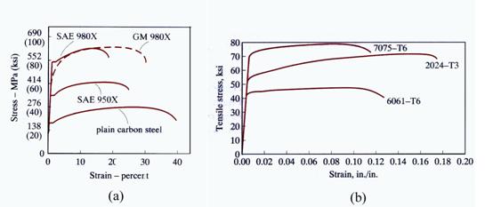 Figure
16 Examples of Stress-Strain Diagrams
Figure
16 Examples of Stress-Strain Diagrams
(a) High-Strength Alloy Steels, (b) Aluminum Alloys
Materials, such as structural steel, which undergo large strain before fracture are called ductile materials. The ductility factor is represented by the ratio of the strain measured at rupture (point G) and that corresponding to the point B in Figure 15. For metals used in structural engineering the ductility factor can reach values between 10 and 20.
The materials which fail at small strain value are called brittle materials. A qualitative difference between a ductile and brittle material are shown in Figure 17. Typical examples of brittle behavior are the following materials: ceramics, glass, cast iron. The welding material, when the weld is improperly made, also exhibits brittle behavior which in many cases compromises the quality of the entire structural ensemble. Drastic change in temperature, pressure and load application can very much influence the material behavior.
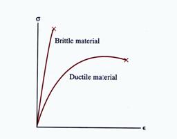
Figure 17 Ductile and Brittle Stress-Strain Diagrams
The temperature is an important factor in the material behavior. Same materials can change from ductile to brittle behavior as a function of the temperature.
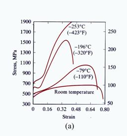
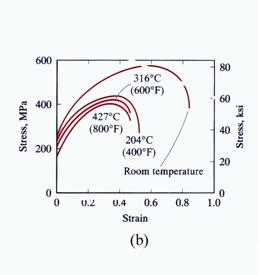
Figure 18 Variation of the Stress-Strain Diagram with Temperature
(a) Low Temperature, (b) High Temperature
In most common applications the materials used in structural engineering are not subjected to temperature extremes great enough to adversely affect the ductile behavior. For the special situations when the material is subjected to high or low temperature corresponding stress-strain diagrams must be constructed. Figures 18.a and 18.b illustrate the variation of the stress-strain diagram with temperature for a type of stainless steel. Note that the strain increases for a given stress with increase in temperature and vice versa.
The American Society of Mechanical Engineers (ASME) publishes a handbook containing a large range of stress-strain diagrams for different metal composition and temperatures.
7.3 Elasticity, Plasticity and Creep
The stress-strain diagram described above has been obtained experimentally by continuous loading of the specimen. If at some time during the loading the load applied to the specimen is reversed, theoretically following the same increments as were used during loading, the process is called un-loading.
If the un-loading stress-strain diagram follows the same path as the loading branch the material is said to be an elastic material. Obviously, the elasticity of the material is manifested only if the un-loading occurs before the stress and strain reach the elastic limit, represented by the stress-strain point C shown in Figure 19.
As described previously for a typical structural steel, the stress is proportional to strain (the modulus of elasticity has a constant value) and the behavior is called linear-elastic. There are materials characterized by a nonlinear-elastic behavior. An example of non-linear elastic material is shown in Figure 19.
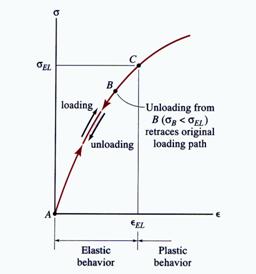
Figure 19 Non-Linear Elastic Behavior
If the stress-strain values corresponding to point C are exceeded the material exhibits a plastic behavior and is said to undergo a plastic flow. A typical loading and un-loading cycle from a plastic range is schematically shown in Figure 20. Noted that during un-loading the material behave as a linear-elastic material.
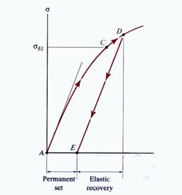
Figure 20 Plastic Behavior
For theoretical applications, the stress-strain diagram shown in Figure 15 is replaced by an artificial but useful stress-strain diagram named Prandtls diagram. This type of diagram is shown in Figure 21 and represents a material with a linear-elastic and perfectly plastic behavior.
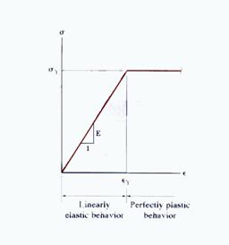
Figure 21 Prandtls Stress-Strain Diagram
The experimental loading and un-loading of the specimen being discussed here are conducted in a relatively short time interval (a few minutes). An interesting phenomenon occurs if the specimen is loaded and then left under a constant load for a long period of time. If the initial strain in the specimen is calculated and the calculation is repeated at intervals of a few days, an increase in the strain is observed. This phenomenon is called creep. The result of a creep experiment is shown in Figure 2
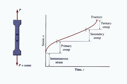
Figure 22 Creep
Similarly, if the specimen is kept under constant strain for a long period of time a reduction in the stress value can be observed. This phenomenon is known as relaxation. A relaxation diagram is depicted in Figure 23.
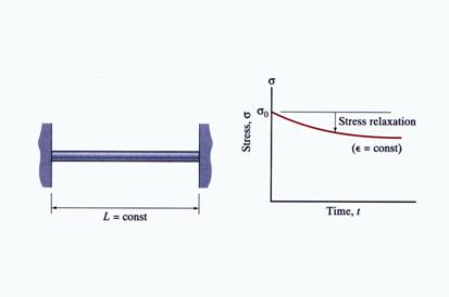
Figure 23 Relaxation
7.4 Linear Elasticity, Hooks Law and Poissons Ratio
The elastic behavior of materials is important for the structural engineering point of view. From the explanations regarding the stress-strain diagram it is clear that if the material is loaded beyond the elastic limit permanent deformations will be present in the solid body. In general, structural engineers design their structures to behave elastically.
Analyzing the stress-strain diagram interval between points A and B illustrated in Figure 15 the proportionality between the stress and strain is evident. Mathematically, the relationship is expressed as:
![]() for
for ![]() (56)
(56)
Equation (56) is
known as Hooks law. As noted earlier,
the constant ![]() is named modulus of
elasticity or Youngs modulus. Structural steels typically have modulus of
elasticity varying around the value of 30000 ksi or 210 GPa.
is named modulus of
elasticity or Youngs modulus. Structural steels typically have modulus of
elasticity varying around the value of 30000 ksi or 210 GPa.
During the elongation of the tensile specimen, a reduction of the dimensions in the other two directions normal to the deformation direction is observed. This transversal contraction, mathematically represented by equation (57), is illustrated in Figure 24 at an exaggerated scale:
![]() (57)
(57)
The constant ![]() is called Poissons ratio. This constant is non-dimensional
and varies for structural steel around the value of 1/3 value. Theoretically,
the Poissons ratio is limited to 0.5. The limits of the Poissons ratio are
treated in Section 5.4.3.
is called Poissons ratio. This constant is non-dimensional
and varies for structural steel around the value of 1/3 value. Theoretically,
the Poissons ratio is limited to 0.5. The limits of the Poissons ratio are
treated in Section 5.4.3.
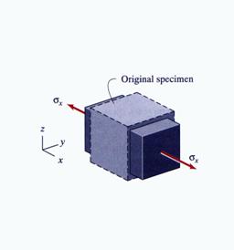
Figure 24 Elongation and Transversal Contraction
7.5 Generalized Hooks Law for Isotropic Materials
The relationship
between stress and strain described for the simple case of uni-axial elongation
will be extended to the general case involving generalized stress and strain
generalized tensors. The material constants ![]() and
and ![]() , together with the thermal coefficient of expansion
, together with the thermal coefficient of expansion ![]() are the most relevant
material characteristics.
are the most relevant
material characteristics.
Figure 25 depicts the general case of the three-axial elongation. Under the influence of applied load and temperature change, the total extensional deformation can be decomposed into four independent effect components: (a) the deformation resulting from the change in temperature, (b), (c) and (d) deformations due to individual application of the three-directional normal stresses. This approach is called the Principle of Linear Superposition.
Note: The Principle of Linear Superposition is discussed in Section 8. The viability of this principle is restricted to the case of small deformation and linear elastic materials.
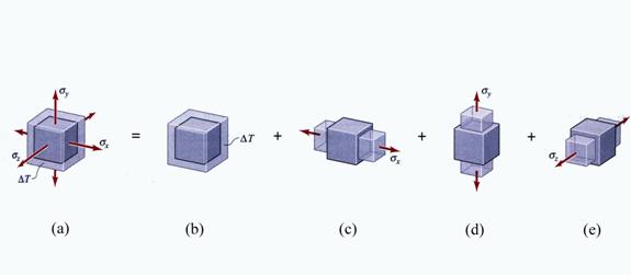
Figure 25 Deformation Induced by a Change in Temperature and
Normal Stress Components
Mathematically, the phenomena illustrated in Figure 25 are described with the following equation:
![]() (57)
(57)
![]() (58)
(58)
![]() (59)
(59)
where the notation stands for:
![]() - is the total
elongation strain in
- is the total
elongation strain in ![]() direction;
direction;
![]() - is the elongation
strain induced by the thermal expansion;
- is the elongation
strain induced by the thermal expansion;
![]() - are the elongation
strains induced by the action of the normal strains
- are the elongation
strains induced by the action of the normal strains ![]() , respectively, in the
, respectively, in the ![]() direction
direction
The total strains ![]() and
and ![]() are similarly defined
by substitution of the appropriate subscripts.
are similarly defined
by substitution of the appropriate subscripts.
The existence of
the normal stress ![]() acting along the ox direction (see Figure 25.c)
introduces, as described in the previous section, the following elongation
strains:
acting along the ox direction (see Figure 25.c)
introduces, as described in the previous section, the following elongation
strains:
![]() (60)
(60)
![]() (61)
(61)
![]() (62)
(62)
Analogously, the formulae (60)
through (62) are written for the case when the normal stress ![]() is considered (see
Figure 25.d) as:
is considered (see
Figure 25.d) as:
![]() (63)
(63)
![]() (64)
(64)
![]() (65)
(65)
Considering the
application of the normal stress ![]() depicted in Figure 25.e
the following equations are written:
depicted in Figure 25.e
the following equations are written:
![]() (66)
(66)
![]() (67)
(67)
![]() (68)
(68)
The thermal strains, which are only elongations, are expressed as:
![]() (69)
(69)
where:
![]() - is the coefficient
of thermal expansion;
- is the coefficient
of thermal expansion;
![]() - is the change in
temperature.
- is the change in
temperature.
Introducing the formulae (60) through (69) into (57) through (59) equations (70) through (72) are obtained as:
![]() (70)
(70)
![]() (71)
(71)
![]() (72)
(72)
For the case of the isotropic linear material the shear strains are related to the shear stresses by the following relationships:
![]() (73)
(73)
![]() (74)
(74)
![]() (75)
(75)
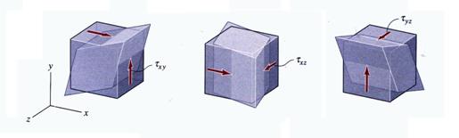
Figure 26 Deformation induced by the Shear Stress Components
Equations (73)
through (75) are illustrated in Figure 26. The constant ![]() is the shear modulus and is obtained from
is the shear modulus and is obtained from ![]() and
and ![]() using the following
relation:
using the following
relation:
![]() (76)
(76)
Equations (70) through (75) are named the Generalized Hooks Law and are widely used in structural engineering applications. By algebraic manipulations equation (70) through (75) may be re-written with the stress tensor components expressed as functions of the strain tensor components. The resulting equations are:
![]() (77)
(77)
![]() (78)
(78)
![]() (79)
(79)
![]() (80)
(80)
![]() (81)
(81)
![]() (82)
(82)
Equations (77) through (82) represent the second form of Hooks law.
8 Fundamental Hypotheses and Equations
The methods employed in Mechanics of Materials are based on three basic hypotheses. They are as follows:
(H1) The solid body is continuous and remains continuous when subjected to exterior actions or changes in temperature;
(H2) Hooks Law;
(H3) There exists a unique unstressed state of body to which the body returns whenever all the exterior actions are removed.
The body satisfying those thee hypotheses is defined as a linear elastic body. Under the hypotheses (H1) the real microscopic atomic structure of the solids is ignored and the solid body is idealized as a geometrical copy in the Euclidian space whose points are identical with the material points of the body. This way the continuity is simulated and no cracks or holes may open in the interior of the solid during the exterior actions. A material satisfying the hypotheses (H1) is called a continuum. The hypotheses (H2) represent the mathematical base of the definition of material elasticity. The direct implication of the Hooks Law is the Principle of Linear Superposition, a principle frequently used in the Mechanics of Materials.
The fundamental concepts presented in the preceding sections are grouped in three fundamental equations extensively used in Mechanics of Materials: (1) the equilibrium equations, (2) the geometry of deformation and (3) the material behavior.
9 Examples
9.1 Stress Distribution and Stress Resultants in a Rectangular Cross-Section
The cross-section
characteristics and the stresses acting on it are depicted in Figure 27. The
origin of the coordinate system ![]() passes though the
center of the rectangular cross-section.
passes though the
center of the rectangular cross-section.
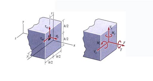
Figure 27 Example 9.1
The stresses existing in the cross-section are expressed by the following functions:
![]() (83)
(83)
![]() (84)
(84)
![]() (85)
(85)
Substituting the relations (83) through (85) into equations (40) through (45) the stress resultant forces and moment are calculated as:
 (86)
(86)
 (87)
(87)
 (88)
(88)
 (89)
(89)
 (90)
(90)
 (91)
(91)
For numeric application the following cross-section dimensions and constant coefficients are assigned:
![]()
![]()
![]()
![]()
![]()
![]()
![]()
![]()
![]()
![]()
![]()
![]()
![]()
![]()
![]()
![]()
The area and the stress resultants obtained by replacing the above values into the equations (86) through (91) are:
![]()
![]()
![]()
![]()
![]()
![]()
![]()
![]()
![]()
![]()
![]()
![]()
![]()
![]()
9.2 Extensional and Shear Strain
The deformation
of a thin square plate with an edge length ![]() is illustrated in
Figure 28. The corner
is illustrated in
Figure 28. The corner![]() moved horizontally by the length
moved horizontally by the length ![]() into a new position
into a new position![]() , while the other three corners kept their original location.
It is supposed that the edge
, while the other three corners kept their original location.
It is supposed that the edge ![]() remains linear through
the deformation.
remains linear through
the deformation.
The extensional
strain in the ![]() direction, accordingly to the definition (46) is:
direction, accordingly to the definition (46) is:
![]() (92)
(92)
To determine
the lengths ![]() and
and![]() two points
two points ![]() and
and ![]() as shown in Figure 28
are selected. After the deformation of the plate they are located in the new
positions
as shown in Figure 28
are selected. After the deformation of the plate they are located in the new
positions ![]() and
and![]() .
.
The original
area of the plate is theoretically divided in both directions in ![]() equally spaced
divisions and the mesh shown in the Figure 28 is obtained. For clarity, in
Figure 28 the number of division was limited only to five (
equally spaced
divisions and the mesh shown in the Figure 28 is obtained. For clarity, in
Figure 28 the number of division was limited only to five (![]() ). The point
). The point ![]() is located at node
is located at node ![]() of the mesh, while the point
of the mesh, while the point ![]() is located at node
is located at node![]() . The original length
. The original length ![]() is obtained as:
is obtained as:
![]() (93)
(93)
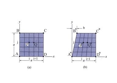
Figure 28 Elongation Strain in Square Plate
(a) Undeformed and (b) Deformed Shapes
After the
deformation the segment ![]() is shorter and is calculated
as:
is shorter and is calculated
as:
 (94)
(94)
The extensional strain is obtained as:
 (95)
(95)
It can be
concluded that the elongation strain ![]() is a function only of variable
is a function only of variable ![]() and varies between values of zero and
and varies between values of zero and ![]() .
.
The shear
strain ![]() which reflects the right angle change is calculated following
a similar rationale. The original right angle is defined by the segments
which reflects the right angle change is calculated following
a similar rationale. The original right angle is defined by the segments ![]() and
and ![]() as shown in Figure 29.a.
After the deformation, as illustrated in Figure 29.b, the angle changes to
angle
as shown in Figure 29.a.
After the deformation, as illustrated in Figure 29.b, the angle changes to
angle ![]() defined between the
segments
defined between the
segments ![]() and
and ![]() .
.
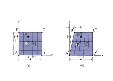
Figure 29 Elongation Strain in Square Plate
(a) Undeformed and (b) Deformed Shapes
From definition 6 the shear strain is given by:
![]() (96)
(96)
The following geometric relations can be written:
![]() (97)
(97)
 (98)
(98)
 (99)
(99)
![]() (100)
(100)
![]() (101)
(101)
The angle ![]() is calculated using
the above formulae:
is calculated using
the above formulae:
 (102)
(102)
The shear strain is obtained as:
![]() (103)
(103)
The shear strain ![]() is dependent only on variable
is dependent only on variable ![]() and varies from
and varies from ![]() to zero value.
to zero value.
9.3 Volumetric Strain
The rectangular parallelepiped of isotropic
linear elastic material is subjected to three normal stresses![]() ,
, ![]() and
and ![]() as shown in Figure 30.
as shown in Figure 30.
The absence of
the shear stress indicates that only volumetric changes result without shape
change. Consequently, the undeformed volume ![]() is modified and after
the deformation the solid body has a new volume
is modified and after
the deformation the solid body has a new volume![]() . The volumetric deformation is called dilatation. The volumetric strain is defined by the following
ratio:
. The volumetric deformation is called dilatation. The volumetric strain is defined by the following
ratio:
![]() (104)
(104)
Using the notation shown in Figure 30 the following relations are written:
![]() (105)
(105)
![]() (106)
(106)
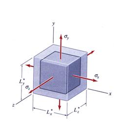
Figure 30 Volumetric Strain
The change in the dimensions is expressed as:
![]() (107)
(107)
![]() (108)
(108)
![]() (109)
(109)
Substituting the above expressions into the expression of the volumetric strain the following equation is obtained:
 (110)
(110)
If the strains are small the products can be neglected and the volumetric strain becomes:
![]() (111)
(111)
Substituting the strain equations
(70) through (72) into equation (111) and for the condition ![]() the volumetric strain
is written as a function of stresses:
the volumetric strain
is written as a function of stresses:
![]() (112)
(112)
Equation (112) indicates that the volumetric strain is always a positive value in the presence of three dimensional tensions, which geometrically represents a volume increase.
|
Politica de confidentialitate | Termeni si conditii de utilizare |

Vizualizari: 4419
Importanta: ![]()
Termeni si conditii de utilizare | Contact
© SCRIGROUP 2026 . All rights reserved