| CATEGORII DOCUMENTE |
| Bulgara | Ceha slovaca | Croata | Engleza | Estona | Finlandeza | Franceza |
| Germana | Italiana | Letona | Lituaniana | Maghiara | Olandeza | Poloneza |
| Sarba | Slovena | Spaniola | Suedeza | Turca | Ucraineana |
For Phenomenological Laws
0. Introduction
A long tradition distinguishes fundamental from phenomenological laws, and favours the fundamental. Fundamental laws are true in themselves; phenomenological laws hold only on account of more fundamental ones. This view embodies an extreme realism about the fundamental laws of basic explanatory theories. Not only are they true (or would be if we had the right ones), but they are, in a sense, more true than the phenomenological laws that they explain. I urge just the reverse. I do so not because the fundamental laws are about unobservable entities and processes, but rather because of the nature of theoretical explanation itself. As I have often urged in earlier essays, like Pierre Duhem, I think that the basic laws and equations of our fundamental theories organize and classify our knowledge in an elegant and efficient manner, a manner that allows us to make very precise calculations and predictions. The great explanatory and predictive powers of our theories lies in their fundamental laws. Nevertheless the content of our scientific knowledge is expressed in the phenomenological laws.
Suppose that some fundamental laws are used to explain a phenomenological law. The ultra-realist thinks that the phenomenological law is true because of the more fundamental laws. One elementary account of this is that the fundamental laws make the phenomenological laws true. The truth of the phenomenological laws derives from the truth of the fundamental laws in a quite literal sensesomething like a causal relation exists between them. This is the view of the seventeenth-century mechanical philosophy of Robert Boyle and Robert Hooke. When God wrote the Book of Nature, he inscribed the fundamental laws of mechanics and he laid down the initial distribution of matter in the universe. Whatever phenomenological laws would be true fell out as a consequence. But this is not only the view of
the seventeenth-century mechanical philosophy. It is a view that lies at the heart of a lot of current-day philosophy of scienceparticularly certain kinds of reductionismand I think it is in part responsible for the widespread appeal of the deductive-nomological model of explanation, though certainly it is not a view that the original proponents of the D-N model, such as Hempel, and Grnbaum, and Nagel, would ever have considered. I used to hold something like this view myself, and I used it in my classes to help students adopt the D-N model. I tried to explain the view with two stories of creation.
Imagine that God is about to write the Book of Nature with Saint Peter as his assistant. He might proceed in the way that the mechanical philosophy supposed. He himself decided what the fundamental laws of mechanics were to be and how matter was to be distributed in space. Then he left to Saint Peter the laborious but unimaginative task of calculating what phenomenological laws would evolve in such a universe. This is a story that gives content to the reductionist view that the laws of mechanics are fundamental and all the rest are epi-phenomenal.
On the other hand, God may have had a special concern for what regularities would obtain in nature. There were to be no distinctions among laws: God himself would dictate each and every one of themnot only the laws of mechanics, but also the laws of chemical bonding, of cell physiology, of small group interactions, and so on. In this second story Saint Peter's task is far more demanding. To Saint Peter was left the difficult and delicate job of finding some possible arrangement of matter at the start that would allow all the different laws to work together throughout history without inconsistency. On this account all the laws are true at once, and none are more fundamental than the rest.
The different roles of God and Saint Peter are essential here: they make sense of the idea that, among a whole collection of laws every one of which is supposed to be true, some are more basic or more true than others. For the seventeenth-century mechanical philosophy, God and the Book of Nature were legitimate devices for thinking of laws and the relations among them. But for most of us nowadays these stories are
mere metaphors. For a long time I used the metaphors, and hunted for some non-metaphorical analyses. I now think that it cannot be done. Without God and the Book of Nature there is no sense to be made of the idea that one law derives from another in nature, that the fundamental laws are basic and that the others hold literally on account of the fundamental ones.
Here the D-N model of explanation might seem to help. In order to explain and defend our reductionist views, we look for some quasi-causal relations among laws in nature. When we fail to find any reasonable way to characterize these relations in nature, we transfer our attention to language. The deductive relations that are supposed to hold between the laws of a scientific explanation act as a formal-mode stand-in for the causal relations we fail to find in the material world. But the D-N model itself is no argument for realism once we have stripped away the questionable metaphysics. So long as we think that deductive relations among statements of law mirror the order of responsibility among the laws themselves, we can see why explanatory success should argue for the truth of the explaining laws. Without the metaphysics, the fact that a handful of elegant equations can organize a lot of complex information about a host of phenomenological laws is no argument for the truth of those equations. As I urged in the last essay, we need some story about what the connection between the fundamental equations and the more complicated laws is supposed to be. There we saw that Adolf Grnbaum has outlined such a story. His outline I think coincides with the views of many contemporary realists. Grnbaum's view eschews metaphysics and should be acceptable to any modern empiricist. Recall that Grnbaum says:
It is crucial to realize that while (a more comprehensive law) G entails (a less comprehensive law) L logically, thereby providing an explanation of L, G is not the cause of L. More specifically, laws are explained not by showing the regularities they affirm to be products of the operation of causes but rather by recognizing their truth to be special cases of more comprehensive truths.1
102
I call this kind of account of the relationship between fundamental and phenomenological laws a generic-specific account. It holds that in any particular set of circumstances the fundamental explanatory laws and the phenomenological laws that they explain both make the same claims. Phenomenological laws are what the fundamental laws amount to in the circumstances at hand. But the fundamental laws are superior because they state the facts in a more general way so as to make claims about a variety of different circumstances as well.
The generic-specific account is nicely supported by the deductive-nomological model of explanation: when fundamental laws explain a phenomenological law, the phenomenological law is deduced from the more fundamental in conjunction with a description of the circumstances in which the phenomenological law obtains. The deduction shows just what claims the fundamental laws make in the circumstances described.
But explanations are seldom in fact deductive, so the generic-specific account gains little support from actual explanatory practice. Wesley Salmon2 and Richard Jeffrey,3 and now many others, have argued persuasively that explanations are not arguments. But their views seem to bear most directly on the explanations of single events; and many philosophers still expect that the kind of explanations that we are concerned with here, where one law is derived from others more fundamental, will still follow the D-N form. One reason that the D-N account often seems adequate for these cases is that it starts looking at explanations only after a lot of scientific work has already been done. It ignores the fact that explanations in physics generally begin with a model. The calculation of the small signals properties of amplifiers, which I discuss in the next section, is an example.4 We first
103
decide which model to useperhaps the T-model, perhaps the hybrid-π model. Only then can we write down the equations with which we will begin our derivation.
Which model is the right one? Each has certain advantages and disadvantages. The T-model approach to calculating the midband properties of the CE stage is direct and simple, but if we need to know how the CE stage changes when the bias conditions change, we would need to know how all the parameters in the transistor circuit vary with bias. It is incredibly difficult to produce these results in a T-model. The T-model also lacks generality, for it requires a new analysis for each change in configuration, whereas the hybrid-π model approach is most useful in the systematic analysis of networks. This is generally the situation when we have to bring theory to bear on a real physical system like an amplifier. For different purposes, different models with different incompatible laws are best, and there is no single model which just suits the circumstances. The facts of the situation do not pick out one right model to use.
I will discuss models at length in the next few essays. Here I want to lay aside my worries about models, and think about how derivations proceed once a model has been chosen. Proponents of the D-N view tend to think that at least then the generic-specific account holds good. But this view is patently mistaken when one looks at real derivations in physics or engineering. It is never strict deduction that takes you from the fundamental equations at the beginning to the phenomenological laws at the end. Instead we require a variety of different approximations. In any field of physics there are at most a handful of rigorous solutions, and those usually for highly artificial situations. Engineering is worse.
Proponents of the generic-specific account are apt to think that the use of approximations is no real objection to their view. They have a story to tell about approximations: the process of deriving an approximate solution parallels a D-N explanation. One begins with some general equations which we hold to be exact, and a description of the situation to which they apply. Often it is difficult, if not impossible, to solve these equations rigorously, so we rely on our description of the situation to suggest approximating procedures.
104
In these cases the approximate solution is just a stand-in. We suppose that the rigorous solution gives the better results; but because of the calculational difficulties, we must satisfy ourselves with some approximation to it.
Sometimes this story is not far off. Approximations occasionally work just like this. Consider, for example, the equation used to determine the equivalent air speed, V E , of a plane (where P T is total pressure, P 0 is ambient pressure, ρ S is sea level density, and M is a Mach number):
The value for V E determined by this equation is close to the plane's true speed.
Approximations occur in connection with (6.1) in two distinct but typical ways. First, the second term,
is significant only as the speed of the plane approaches Mach One. If M < 0.5, the second term is discarded because the result for V E given by
will differ insignificantly from the result given by (6.1). Given this insignificant variation, we can approximate V E by using
for M < 0.5. Secondly, (6.1) is already an approximation, and not an exact equation. The term
has other terms in the denominator. It is a
in the denominator, and so on. For Mach numbers less than one, the error that results from ignoring this third term is less than one per cent, so we truncate and use only two terms.
Why does the plane travel with a velocity, V, roughly equal to
Because of equation (6.1). In fact the plane is really travelling at a speed equal to
But since M is less than 0.5, we do not notice the difference. Here the derivation of the plane's speed parallels a covering law account. We assume that equation (6.1) is a true law that covers the situation the plane is in. Each step away from equation (6.1) takes us a little further from the true speed. But each step we take is justified by the facts of the case, and if we are careful, we will not go too far wrong. The final result will be close enough to the true answer.
This is a neat picture, but it is not all that typical. Most cases abound with problems for the generic-specific account. Two seem to me especially damaging: (1) practical approximations usually improve on the accuracy of our fundamental laws. Generally the doctored results are far more accurate than the rigorous outcomes which are strictly implied by the laws with which we begin. (2) On the generic-specific account the steps of the derivation are supposed to show how the fundamental laws make the same claims as the phenomenological laws, given the facts of the situation. But seldom are the facts enough to justify the derivation. Where approximations are called for, even a complete knowledge of the circumstances may not provide the additional premises necessary to deduce the phenomenological laws from the fundamental equations that explain them. Choices must be
106
made which are not dictated by the facts. I have already mentioned that this is so with the choice of models. But it is also the case with approximation procedures: the choice is constrained, but not dictated by the facts, and different choices give rise to different, incompatible results. The generic-specific account fails because the content of the phenomenological laws we derive is not contained in the fundamental laws which explain them.
These two problems are taken up in turn in the next two sections. A lot of the argumentation, especially in Section 2, is taken from a paper written jointly by Jon Nordby and me, How Approximations Take Us Away from Theory and Towards the Truth.5 This paper also owes a debt to Nordby's Two Kinds of Approximations in the Practice of Science.6
1. Approximations That Improve on Laws
On the generic-specific account, any approximation detracts from truth. But it is hard to find examples of this at the level where approximations connect theory with reality, and that is where the generic-specific account must work if it is to ensure that the fundamental laws are true in the real world. Generally at this level approximations take us away from theory and each step away from theory moves closer towards the truth. I illustrate with two examples from the joint paper with Jon Nordby.
1.1. An Amplifier Model
Consider an amplifier constructed according to Figure 6.1. As I mentioned earlier, there are two ways to calculate the small signal properties of this amplifier, the T-model and the hybrid-π model. The first substitutes a circuit model for the transistor and analyses the resulting network. The second characterizes the transistor as a set of two-port parameters and calculates the small signal properties of the amplifier
107
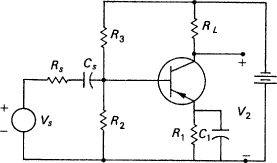
Fig. 6.1
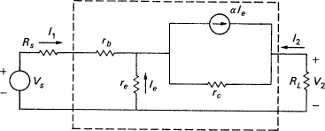
Fig. 6.2
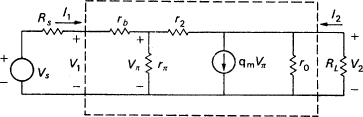
Fig. 6.3
in terms of these parameters. The two models are shown in Figures 6.2 and 6.3 inside the dotted area.
The application of these transistor models in specific situations gives a first rough approximation of transistor parameters at low frequencies. These parameters can be theoretically estimated without having to make any measurements on the actual circuit. But the theoretical estimates are often grossly inaccurate due to specific causal features present in the actual circuit, but missing from the models.
108
One can imagine handling this problem by constructing a larger, more complex model that includes the missing causal features. But such a model would have to be highly specific to the circuit in question and would thus have no general applicability.
Instead a different procedure is followed. Measurements of
the relevant parameters are made on the actual circuit under study, and then
the measured values rather than the theoretically predicted values are used for
further calculations in the original models. To illustrate, consider an actual
amplifier, built and tested such that I E =1 ma; R
L = 2.7 ![]() 15 =
2.3 k ohm; R 1 = 1 k ohm. β = 162 and R S
= 1 k ohm and assume r b = 50 ohms. The theoretical
expectation of midband gain is
15 =
2.3 k ohm; R 1 = 1 k ohm. β = 162 and R S
= 1 k ohm and assume r b = 50 ohms. The theoretical
expectation of midband gain is
The actual measured midband gain for this amplifier with an output voltage at f = 2 kHz and source voltage at 1.8 mv and 2 kHz, is
This result is not even close to what theory predicts. This fact is explained causally by considering two features of the situation: first, the inaccuracy of the transistor model due to some undiagnosed combination of causal factors; and second, a specifically diagnosed omissionthe omission of equivalent series resistance in the bypass capacitor. The first inaccuracy involves the value assigned to r e by theory. In theory, r e = kT/qI E , which is approximately 25.9/I E . The actual measurements indicate that the constant of proportionality for this type of transistor is 30 mv, so r e = 30/I E , not 25.9/I E .
Secondly, the series resistance is omitted from the ideal capacitor. But real electrolytic capacitors are not ideal. There is leakage of current in the electrolyte, and this can be modelled by a resistance in series with the capacitor. This series resistance is often between 1 and 10 ohms, sometimes as high as 25 ohms. It is fairly constant at low frequency but
109
increases with increased frequency and also with increased
temperature. In this specific case, the series resistance, ![]() ,
is measured as 12 ohms.
,
is measured as 12 ohms.
We must now modify (6.3) to account for these features, given our measured result in (6.4) of A V , meas. = 44:
Solving this equation gives us a predicted midband gain of 47.5, which is sufficiently close to the measured midband gain for most purposes.
Let us now look back to see that this procedure is very different from what the generic-specific account supposes. We start with a general abstract equation, (6.3); make some approximations; and end with (6.5), which gives rise to detailed phenomenological predictions. Thus superficially it may look like a D-N explanation of the facts predicted. But unlike the covering laws of D-N explanations, (6.3) as it stands is not an equation that really describes the circuits to which it is applied. (6.3) is refined by accounting for the specific causal features of each individual situation to form an equation like (6.5). (6.5) gives rise to accurate predictions, whereas a rigorous solution to (6.3) would be dramatically mistaken.
But one might object: isn't the circuit model, with no
resistance added in, just an idealization? And what harm is that? I agree that
the circuit model is a very good example of one thing we typically mean by the
term idealization. But how can that help the defender of fundamental
laws? Most philosophers have made their peace with idealizations: after all, we
have been using them in mathematical physics for well over two thousand years.
Aristotle in proving that the rainbow is no greater than a semi-circle in Meterologica
III. 5 not only treats the sun as a point, but in a blatant falsehood puts the
sun and the reflecting medium (and hence the rainbow itself) the same distance
from the observer. Today we still make the same kinds of idealizations in our
celestial theories. Nevertheless, we have managed to discover the planet
But what solace is this to the realist? How do idealizations save the truth of the fundamental laws? The idea seems to be this. To call a model an idealization is to suggest that the model is a simplification of what occurs in reality, usually a simplification which omits some relevant features, such as the extended mass of the planets or, in the example of the circuit model, the resistance in the bypass capacitor. Sometimes the omitted factors make only an insignificant contribution to the effect under study. But that does not seem to be essential to idealizations, especially to the idealizations that in the end are applied by engineers to study real things. In calling something an idealization it seems not so important that the contributions from omitted factors be small, but that they be ones for which we know how to correct. If the idealization is to be of use, when the time comes to apply it to a real system we had better know how to add back the contributions of the factors that have been left out. In that case the use of idealizations does not seem to counter realism: either the omitted factors do not matter much, or in principle we know how to treat them.
In the sense I just described, the circuit model is patently an idealization. We begin with equation (6.3), which is inadequate; we know the account can be improvedNordby and I show how. But the improvements come at the wrong place for the defender of fundamental laws. They come from the ground up, so-to-speak, and not from the top down. We do not modify the treatment by deriving from our theoretical principles a new starting equation to replace (6.3). It is clear that we could not do so, since only part of the fault is diagnosed. What we do instead is to add a phenomenological correction factor, a factor that helps produce a correct description, but that is not dictated by fundamental law.
But could we not in principle make the corrections right at the start, and write down a more accurate equation from the beginning? That is just the assumption I challenge. Even if we could, why do we think that by going further and further backwards, trying to get an equation that will be right when all the significant factors are included, we will eventually
111
get something simple which looks like one of the fundamental laws of our basic theories? Recall the discussion of cross-effects from Essay 3. There I urged that we usually do not have any uniform procedure for adding interactions. When we try to write down the more correct equations, we get a longer and longer list of complicated laws of different forms, and not the handful of simple equations which could be fundamental in a physical theory.
Generality and simplicity are the substance of explanation. But they are also crucial to application. In engineering, one wants laws with a reasonably wide scope, models that can be used first in one place then another. If I am right, a law that actually covered any specific case, without much change or correction, would be so specific that it would not be likely to work anywhere else. Recall Bertrand Russell's objection to the same cause, same effect principle:
The principle same cause, same effect, which philosophers imagine to be vital to science, is therefore utterly otiose. As soon as the antecedents have been given sufficiently fully to enable the consequents to be calculated with some exactitude, the antecedents have become so complicated that it is very unlikely they will ever recur. Hence, if this were the principle involved, science would remain utterly sterile.8
Russell's solution is to move to functional laws which state relations between properties (rather than relations between individuals). But the move does not work if we want to treat real, complex situations with precision. Engineers are comfortable with functions. Still they do not seem able to find functional laws that allow them to calculate consequences with some exactitude and yet are not so complicated that it is very unlikely they will ever recur. To find simple laws that we can use again and again, it looks as if we had better settle for laws that patently need improvement. Following Russell, it seems that if we model approximation on D-N explanation, engineering would remain utterly sterile.
112
1.2 Exponential Decay
The second example concerns the derivation of the exponential decay law in quantum mechanics. I will describe this derivation in detail, but the point I want to stress can be summarized by quoting one of the best standard texts, by Eugen Merzbacher: The fact remains that the exponential decay law, for which we have so much empirical support in radioactive processes, is not a rigorous consequence of quantum mechanics but the result of somewhat delicate approximations.9
The exponential decay law is a simple, probabilistically elegant law, for whichas Merzbacher sayswe have a wealth of experimental support. Yet it cannot be derived exactly in the quantum theory. The exponential law can only be derived by making some significant approximation. In the conventional treatment the rigorous solution is not pure exponential, but includes several additional terms. These additional terms are supposed to be small, and the difference between the rigorous and the approximate solution will be unobservable for any realistic time periods. The fact remains that the data, together with any reasonable criterion of simplicity (and some such criterion must be assumed if we are to generalize from data to laws at all) speak for the truth of an exponential law; but such a law cannot be derived rigorously. Thus it seems that the approximations we make in the derivation take us closer to, not further from, the truth.
There are two standard treatments of exponential decay: the WeisskopfWigner treatment, which was developed in their classic paper of 1930,10 and the more recent Markov treatment, which sees the exponential decay of an excited atom as a special case in the quantum theory of damping. We will look at the more recent treatment first. Here we consider an abstract system weakly coupled to a reservoir. The aim is to derive a general master equation for the
113
evolution of the system. This equation is similar to the evolution equations of classical statistical mechanics. For the specific case in which we are interested, where the system is an excited atom and the reservoir the electromagnetic field, the master equation turns into the Pauli rate equation, which is the analogue of the exponential law when re-excitement may occur:
Pauli equation:
(Here S j is the occupation probability of the jth state; Γ j , the inverse of the lifetime; and ω jk is the transition probability from state k to state j.)
The derivation of the master equation is quite involved. I will focus on the critical feature from my point of viewthe Markov approximation. Generally such a derivation begins with the standard second-order perturbation expansion for the state x of the composite, system and reservoir, which in the interaction picture looks like this:
Notice that the state of the system and reservoir at t depends on its entire past history through the integrals on the right-hand side of this equation. The point of the Markov approximation is to derive a differential equation for the state of the system alone such that the change in this state at a time depends only on the facts about the system at that time, and not on its past history. This is typically accomplished by two moves: (i) extending the time integrals which involve only reservoir correlations to infinity, on the grounds that the correlations in the reservoir are significant for only a short period compared to the periods over which we are observing the system; and (ii) letting t − t 0 → 0, on the grounds that the periods of time considered for the system are small compared to its lifetime. The consequence is a master equation
114
with the desired feature. As W. H. Louisell remarks in his chapter on damping:
We note that the r.h.s. [right hand side] of [the master equation] no longer contains time integrals over S(t′) [S is the state of the system alone] for times earlier than the present so that the future is now indeed determined by the present. We have assumed that the reservoir correlation times are zero on a time scale in which the system loses an appreciable amount of its energy . . . One sometimes refers to the Markoff approximation as a coarse-grained averaging.11
Thus the Markov approximation gives rise to the master equation; for an atom in interaction with the electromagnetic field, the master equation specializes to the Pauli equation; and the Pauli equation predicts exponential decay for the atom. Without the Markov approximation, the decay can at best be near exponential.
Let us now look at the WeisskopfWigner method, as it is employed nowadays. We begin with the exact Schroedinger equations for the amplitudes, but assume that the only significant coupling is between the excited and the de-excited states:
(ω eg is ![]() ,
for E e the energy of the excited state, E g
the energy of the de-excited; ω f is the frequency of
the fth mode of the field; and g ef is the
coupling constant between the excited state and the fth mode. c e
is the amplitude in the excited state, no photons present.)
,
for E e the energy of the excited state, E g
the energy of the de-excited; ω f is the frequency of
the fth mode of the field; and g ef is the
coupling constant between the excited state and the fth mode. c e
is the amplitude in the excited state, no photons present.)
The first approximation notes that the modes of the field available to the de-exciting atom form a near continuum. (We will learn more about this in the next section.) So the sum over f can be replaced by an integral, to give
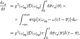
or setting γ ≡ 2πg2(ω eg ) 𝓓 (ω eg ),
and finally,
But in moving so quickly we lose the Lamb shifta small displacement in the energy levels discovered by Willis Lamb and R. C. Retherford in 1947. It will pay to do the integrals in the opposite order. In this case, we note that c e (t) is itself slowly varying compared to the rapid oscillations from the exponential, and so it can be factored out of the t′ integral, and the upper limit of that integral can be extended to infinity. Notice that the extension of the t′ limit is very similar to the Markov approximation already described, and the rationale is similar. We get
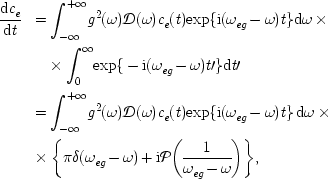
or, setting γ ≡ 2πg2(ω eg )𝓓(ω eg ) and
116
(𝓟(x) = principal part ofx.)
Here Δω is the Lamb shift. The second method, which results in a Lamb shift as well as the line-broadening γ, is what is usually now called the WeisskopfWigner method.
We can try to be more formal and avoid approximation
altogether. The obvious way to proceed is to evaluate the
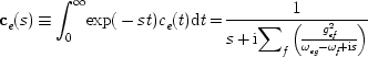
then
To solve this equation, the integrand must be defined on the first and second Riemann sheets. The method is described clearly in Goldberger and Watson's text on collision theory.12
The primary contribution will come from a simple pole Δ![]() such
that
such
that
This term will give us the exponential we want:
But this is not an exact solution. As we distort the contour
on the Riemann sheets, we cross other poles which we have not yet considered.
We have also neglected the integral around the final contour itself. Goldberger
and Watson calculate that this last integral contributes a term proportional to
![]() .
They expect that the other poles will add only
.
They expect that the other poles will add only
117
negligible contributions as well, so that the exact answer will be a close approximation to the exponential law we are seeking; a close approximation, but still only an approximation. If a pure exponential law is to be derived, we had better take our approximations as improvements on the initial Schroedinger equation, and not departures from the truth.
Is there no experimental test that tells which is right? Is decay really exponential, or is the theory correct in predicting departures from the exponential law when t gets large? There was a rash of tests of the experimental decay law in the middle 1970s, spurred by E. T. Jaynes's neo-classical theory of the interaction of matter with the electromagnetic field, a theory that did surprisingly well at treating what before had been thought to be pure quantum phenomena. But these tests were primarily concerned with Jaynes's claim that decay rates would depend on the occupation level of the initial state. The experiments had no bearing on the question of very long time decay behaviour. This is indeed a very difficult question to test. Rolf Winter13 has experimented on the decay of Mn56 up to 34 half-lives, and D. K. Butt and A. R. Wilson on the alpha decay of radon for over 40 half-lives.14 But, as Winter remarks, these lengths of time, which for ordinary purposes are quite long, are not relevant to the differences I have been discussing, since for the radioactive decay of Mn56. . . non-exponential effects should not occur before roughly 200 half-lives. In this example, as with all the usual radioactive decay materials, nothing observable should be left long before the end of the exponential region.15 In short, as we read in a 1977 review article by A. Pais, experimental situations in which such deviations play a role have not been found to date.16 The times before the differences emerge are just too long.
118
2. Approximations not Dictated by the Facts
Again, I will illustrate with two examples. The examples show how the correct approximation procedure can be undetermined by the facts. Both are cases in which the very same procedure, justified by exactly the same factual claims, gives different results depending on when we apply it: the same approximation applied at different points in the derivation yields two different incompatible predictions. I think this is typical of derivation throughout physics; but in order to avoid spending too much space laying out the details of different cases, I will illustrate with two related phenomena: (a) the Lamb shift in the excited state of a single two-level atom; and (b) the Lamb shift in the ground state of the atom.
2.1. The Lamb Shift in the Excited State
Consider again spontaneous emission from a two-level atom. The traditional way of treating exponential decay derives from the classic paper of V. Weisskopf and Eugene Wigner in 1930, which I described in the previous section. In its present form the WeisskopfWigner method makes three important approximations: (1) the rotating wave approximation; (2) the replacement of a sum by an integral over the modes of the electromagnetic field and the factoring out of terms that vary slowly in the frequency; and (3) factoring out a slowly-varying term from the time integral and extending the limit on the integral to infinity. I will discuss the first approximation below when we come to consider the level shift in the ground state. The second and third are familiar from the last section. Here I want to concentrate on how they affect the Lamb shift in the excited state.
Both approximations are justified by appealing to the physical characteristics of the atom-field pair. The second approximation is reasonable because the modes of the field are supposed to form a near continuum; that is, there is a very large number of very closely spaced modes. This allows us to replace the sum by an integral. The integral is over a product of the coupling constant as a function of the frequency, ω, and a term of the form exp(−iωt). The coupling
119
constant depends on the interaction potential for the atom and the field, and it is supposed to be relatively constant in ω compared to the rapidly oscillating exponential. Hence it can be factored outside the integral with little loss of accuracy. The third approximation is similarly justified by the circumstances.
What is important is that, although each procedure is separately rationalized by appealing to facts about the atom and the field, it makes a difference in what order they are applied. This is just what we saw in the last section. If we begin with the third approximation, and perform the t integral before we use the second approximation to evaluate the sum over the modes, we predict a Lamb shift in the excited state. If we do the approximations and take the integrals in the reverse orderwhich is essentially what Weisskopf and Wigner did in their original paperwe lose the Lamb shift. The facts that we cite justify both procedures, but the facts do not tell us in what order to apply them. There is nothing about the physical situation that indicates which order is right other than the fact to be derived: a Lamb shift is observed, so we had best do first (3), then (2). Given all the facts with which we start about the atom and the field and about their interactions, the Lamb shift for the excited state fits the fundamental quantum equations. But we do not derive it from them.
One may object that we are not really using the same approximation in different orders; for, applied at different points, the same technique does not produce the same approximation. True, the coefficients in t and in ω are slowly varying, and factoring them out of the integrals results in only a small error. But the exact size of the error depends on the order in which the integrations are taken. The order that takes first the t integral and then the ω integral is clearly preferable, because it reduces the error.
Two remarks are to be made about this objection. Both have to do with how approximations work in practice. First, in this case it looks practicable to try to calculate and to compare the amounts of error introduced by the two approximations. But often it is practically impossible to decide which of two procedures will lead to more accurate results. For instance, we often justify dropping terms from an equation by showing that the coefficients of the omitted terms are small compared to those of the terms we retain. But as the next example will show, knowing the relative sizes of terms in the equation is not a sure guide to the exact effects in the solution, particularly when the approximation is embedded in a series of other approximations. This is just one simple case. The problem is widespread. As I argued in Essay 4, proliferation of treatments is the norm in physics, and very often nobody knows exactly how they compare. When the situation becomes bad enough, whole books may be devoted to sorting it out. Here is just one example, The Theory of Charge Exchange by Robert Mapleton. The primary purpose of the book is to explain approximating methods for cross sections and probabilities for electronic capture. But its secondary purpose is
to compare different approximate predictions with each other and with experimentally determined values. These comparisons should enable us to determine which approximating procedures are most successful in predicting cross sections for different ranges . . . they also should indicate which methods show most promise for additional improvement.17
Comparing approximations is often no easy matter.
Secondly, the objection assumes the principle the more accuracy, the better. But this is frequently not so, for a variety of well-known reasons: the initial problem is set only to a given level of accuracy, and any accuracy in the conclusion beyond this level is spurious; or the use of certain mathematical devices, such as complex numbers, will generate excess terms which we do not expect to have any physical significance; and so on. The lesson is this: a finer approximation provides a better account than a rougher one only if the rougher approximation is not good enough. In the case at hand, the finer approximation is now seen to be preferable, not because it produces a quantitatively slightly more accurate treatment, but rather because it exposes a qualitatively significant new phenomenonthe Lamb shift in the ground state. If you look back at the equations in the last section
121
it is obvious that the first-ω-then t order
misses an imaginary term: the amplitude to remain in the excited state has the
form ![]() rather
than
rather
than ![]() .
This additional imaginary term, iω, appears when the integrals are done in
the reverse order, and it is this term that represents the Lamb shift. But what
difference does this term make? In the most immediate application, for
calculating decay probabilities, it is completely irrelevant, for the
probability is obtained by multiplying together the amplitude
.
This additional imaginary term, iω, appears when the integrals are done in
the reverse order, and it is this term that represents the Lamb shift. But what
difference does this term make? In the most immediate application, for
calculating decay probabilities, it is completely irrelevant, for the
probability is obtained by multiplying together the amplitude ![]() ,
and its complex conjugate
,
and its complex conjugate ![]() ,
in which case the imaginary part disappears and we are left with the well-known
probability for exponential decay, exp(−Γt).
,
in which case the imaginary part disappears and we are left with the well-known
probability for exponential decay, exp(−Γt).
The point is borne out historically. The first-ω-then-t order, which loses the Lamb shift, is an equivalent approximation to the ansatz which Weisskopf and Wigner use in their paper of 1930, and it was the absolutely conventional treatment for seventeen years. To calculate the value of the missing imaginary terms, one has to come face to face with divergences that arise from the Dirac theory of the electron, and which are now so notorious in quantum electrodynamics. These problems were just pushed aside until the remarkable experiments in 1947 by Willis Lamb and his student R. C. Retherford, for which Lamb later won the Nobel prize.
The Dirac theory, taking the spin of the electron into account, predicted an exact coincidence of the 22P 1/2 and the 22S 1/2 levels. There was a suspicion that this prediction was wrong. New microwave techniques developed during the war showed Lamb a way to find out, using the metastable 22S 1/2 state of hydrogen. In the 1947 experiment the Lamb shift was discovered and within a month Bethe had figured a way to deal with the divergences. After the discovery of the Lamb shift the original WeisskopfWigner method had to be amended. Now we are careful to take the integrals in the first-t-then-ω order. But look at what Bethe himself has to say:
By very beautiful experiments, Lamb and Retherford have shown that the fine structure of the second quantum state of hydrogen does not agree with the prediction of the Dirac theory. The 2s level, which
122
according to Dirac's theory should coincide with the 2p 1/2 level, is actually higher than the latter by an amount of about 0.033 cm−1 or 1000 megacycles . . .
Schwinger and Weisskopf, and Oppenheimer have suggested that a possible explanation might be the shift of energy levels by the interaction of the electron with the radiation field. This shift comes out infinite in all existing theories, and has therefore always been ignored.18
Or consider Lamb's comment on Bethe in his Nobel Prize address:
A month later [after the fine structure deviations were definitely established experimentally by Lamb and Retherford], Bethe found that quantum electrodynamics had really hidden behind its divergences a physical content that was in very close agreement with the microwave observations.19
Now we attend to the imaginary terms because they have real physical content . . . in very close agreement with microwave observations. But until Lamb's experiments they were just mathematical debris which represented nothing of physical significance and were, correctly, omitted.
2.2. The Lamb Shift in the Ground State
The details of the second example are in G. S. Agarwal's monograph on spontaneous emission.20 Recall that there are two common methods for treating spontaneous emission. The first is the WeisskopfWigner method, and the second is via a Markov approximation, leading to a master equation or a Langevin equation, analogous to those used in classical statistical mechanics. As Agarwal stresses, one reason for preferring the newer statistical approach is that it allows us to derive the Lamb shift in the ground state, which is not predicted by the WeisskopfWigner method even after that method has been amended to obtain the shift in the excited state. But we can derive the ground state shift only if we are careful about how we use the rotating wave approximation.
123
The rotating wave approximation is used when the interaction
between radiation and matter is weak. In weak interactions, such as those that
give rise to spontaneous emission, the atoms and field can be seen as almost
separate systems, so that energy lost by the atoms will be found in the field,
and vice versa. Thus virtual transitions in which both the atom and the field
simultaneously gain or lose a quantum of energy will have negligible effects.
The rotating wave approximation ignores these effects. When the coupling is
weak, the terms which represent virtual transitions vary as
exp ( ![]() ,
for energies levels E m and E n
of the atom; ω k is a mode frequency of the field).
Energy conserving transitions vary as exp. For optical frequencies ω k is large. Thus
for ordinary times of observation the exp terms oscillate rapidly, and will average approximately to zero. The
approximation is called a rotating-wave approximation because it retains only
terms in which the atom and field waves rotate together.
,
for energies levels E m and E n
of the atom; ω k is a mode frequency of the field).
Energy conserving transitions vary as exp. For optical frequencies ω k is large. Thus
for ordinary times of observation the exp terms oscillate rapidly, and will average approximately to zero. The
approximation is called a rotating-wave approximation because it retains only
terms in which the atom and field waves rotate together.
The statistical treatments which give rise to the master equation make an essential use of a Markov approximation. In the last section I outlined one standard way to derive the Pauli equations, which are the master equations relevant for spontaneous emission. But according to Agarwal, there are two ways to carry through such a derivation, and the results are significantly different depending on where we apply the rotating wave approximation. On the one hand, we can begin with the full Hamiltonian for the interaction of the orbiting electron with the electromagnetic field, and drop from this Hamiltonian the counter-rotating terms which represent virtual transitions, to obtain a shortened approximate Hamiltonian which Agarwal numbers (2.24). Then, following through steps like those described above, one obtains a version of the master equationAgarwal's equation A.7. Alternatively, we can use the full Hamiltonian throughout, dropping the counter-rotating terms only in the last step. This gives us Agarwal's equation (A.6).
What difference do the two methods make to the Lamb shift? Agarwal reports:
The shift of the ground state is missing from (A.7), mainly due to the virtual transitions which are automatically excluded from the
124
Hamiltonian (2.24). The master equation (A.6) obtained by making RWA (the rotating wave approximation) on the master equation rather than on the Hamiltonian does include the shift of the ground state. These remarks make it clear that RWA on the original Hamiltonian is not the same as RWA on the master equation and that one should make RWA on the final equations of motion.21
The rotating wave approximation is justified in cases of spontaneous emission by the weakness of the coupling between the atom and the field. But no further features of the interaction determine whether we should apply the approximation to the original Hamiltonian, or whether instead we should apply it to the master equation. Agarwal applies it to the master equation, and he is thus able to derive a Lamb shift in the ground state. But his derivation does not show that the Schroedinger equation dictates a Lamb shift for a two-level atom in weak interaction with an electro-magnetic field. The shift is consistent with what the equation says about weak interactions, but it does not follow from it.
This kind of situation is even more strikingly illustrated if we try to calculate the values of the shifts for the two-level atoms. Lamb and Retherford's experiments, for example, measured the value of the shift for the 2S state in hydrogen to be 1057 mega-cycles per second. We can derive a result very close to this in quantum electrodynamics using the technique of mass renormalization for the electron. But the derivation is notorious: the exact details, in which infinities are subtracted from each other in just the right way to produce a convergent result, are completely ad hoc, and yet the quantitative results that they yield are inordinately accurate.
The realist has a defence ready. I say that the Schroedinger equation does not make a claim about whether there is or is not a Lamb shift in the circumstances described. But the realist will reply that I have not described the circumstances as fully as possible. The rotating wave approximations depend on the fact that the interaction between the field and the atom is weak; but if realism is correct, there is a precise answer to the question How weak? The atom-field interaction will have a precise quantitative representation that can in principle be written into the Schroedinger equation. The exact solution to the equation with that term written in will either contain a Lamb shift, or it will not, and that is what the Schroedinger equation says about a Lamb shift in cases of spontaneous emission.
This defence allows me to state more exactly the aims of this essay. I do not argue against taking the fundamental laws as true, but try only to counter the most persuasive argument in favour of doing so. As a positive argument in favour of realism, the realist's defence, which plumps for exact solutions and rigorous derivations, gets the logic of the debate out of order. I begin with the challenge, Why should we assume that the short abstract equations, which form the core of our fundamental theories, are true at all, even true enough for now? The realist replies Because the fundamental equations are so successful at explaining a variety of messy and complicated phenomenological laws. I say Tell me more about explanation. What is there in the explanatory relation which guarantees that the truth of the explanandum argues for the truth of the explanans? The realist's answer, at least on the plausible generic-specific account, is that the fundamental laws say the same thing as the phenomenological laws which are explained, but the explanatory laws are more abstract and general. Hence the truth of the phenomenological laws is good evidence for the truth of the fundamental laws. I reply to this, Why should we think the fundamental and the phenomenological laws say the same thing about the specific situations studied? and the realist responds, Just look at scientific practice. There you will see that phenomenological laws are deducible from the more fundamental laws that explain them, once a description of the circumstances is given.
We have just been looking in detail at cases of scientific practice, cases which I think are fairly typical. Realists can indeed put a gloss on these examples that brings them into line with realist assumptions: rigorous solutions to exact equations might possibly reproduce the correct phenomenological laws with no ambiguity when the right equations are found. But the reason for believing in this gloss is not the practice itself, which we have been looking at, but rather the realist
126
metaphysics, which I began by challenging. Examples of the sort we have considered here could at best be thought consistent with realist assumptions, but they do not argue for them.
3. Conclusion
Fundamental laws are supposed by many to determine what phenomenological laws are true. If the primary argument for this view is the practical explanatory success of the fundamental laws, the conclusion should be just the reverse. We have a very large number of phenomenological laws in all areas of applied physics and engineering that give highly accurate, detailed descriptions of what happens in realistic situations. In an explanatory treatment these are derived from fundamental laws only by a long series of approximations and emendations. Almost always the emendations improve on the dictates of the fundamental law; and even where the fundamental laws are kept in their original form, the steps of the derivation are frequently not dictated by the facts. This makes serious trouble for the D-N model, the generic-specific account, and the view that fundamental laws are better. When it comes to describing the real world, phenomenological laws win out.
|
Politica de confidentialitate | Termeni si conditii de utilizare |

Vizualizari: 1573
Importanta: ![]()
Termeni si conditii de utilizare | Contact
© SCRIGROUP 2025 . All rights reserved