LINEAR PREDICTION

INTRODUCTION

Wouldnt it be great to pick up tomorrows newspaper and read about prices before they occur? While that isnt possible, perhaps the next best thing is to use the power of your computer to predict what those prices are going to be. We will show you exactly how to make these predictions in this article. The predictive filter we use is adapted from the approach described by Lloyd J. Griffiths . Griffiths uses a simple time-domain gradient algorithm to continually adapt the coefficients of the linear prediction filter. He goes on to make a spectral estimate of the signal in a manner similar to MESA, but that is not the focus of this article.

We describe the linear prediction filter and provide EasyLanguage code to implement it as a price predictor. One of the filter constraints is that the amplitude of the signal be limited to 1. This constraint means the filter is a better predictor of oscillators like the Stochastic and RSI, whose amplitudes are already naturally limited. It turns out that performing a gain limitation on prices introduces a lag in the prediction such that the resulting signals can be used as counter trenders.

LINEAR PREDICTION FILTER

The basic form of a linear prediction filter of length L is shown in Figure 1. The input signal, x[n], is applied to a shift register. Each step of the shift register is delayed one sample period, as denoted by z^-1. The output of each delay step is multiplied by a unique gain factor and summed to form and estimate of x[n], called xBar[L]. Then, the estimate xBar[L] is subtracted from the real input signal, x[n], to obtain the error term e[n]. The algorithm minimizes the error term by adjusting each of the gain terms in a recursive manner, using the error term and a convergence factor. The derivation of the Least Mean Squares (LMS) algorithm to determine the gain terms is of little interest to most traders, and so those readers who are interested in the derivation are referred to Griffiths paper.

Figure 1. Basic form of a linear prediction filter

The convergence factor is called m (Mu). It is represented by the equation

m a / (L*Power[0])

If the Power in the waveform is unity, the convergence factor becomes simply

m a / L

Convergence of the algorithm is assured when 0 < a < 2. I find the best value to be a=.25, but the selection range is very broad.

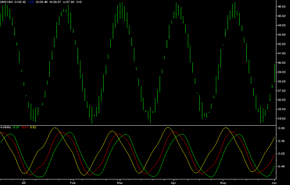
Power in a waveform is proportional to its average squared amplitude. Since the most simple representation of the convergence factor is when the power is unity, this suggests the use of an oscillator such as a Stochastic or RSI since their scaled amplitudes are already limited to unity (and multiplied by 100 to be expressed in terms of percent). It is a simple matter to offset these oscillators to swing about their midpoints to maximum extreme values of +1 and 1. Figure 2 is a 10 Bar Slow Stochastic for a 24 bar theoretical sinewave data (green line), the 2 bar prediction for the Stochastic (red line), and the 5 bar prediction (yellow line). The prediction is nearly perfect in this theoretical example. The signal to buy is when the 2 day prediction crosses over the Stochastic and the signal to sell is when the 2 day prediction crosses under the Stochastic.

Figure2.  Two and Five Bar Predictions of a 24 Bar Cycle Slow Stochastic

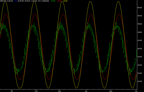
The theoretical sinewave price data swings plus and minus 5 about an average value of 40. If this waveform is to be used in the Griffiths algorithm, then the convergence factor must be normalized to the power in the waveform. It turns out that the normalizer fluctuates during the cycle period in such a way as to introduce lag into the prediction. A zero lag Kalman filter (green line) is shown in Figure 3, along with its 2 bar prediction (red line) and 5 bar prediction (yellow line). Comparing these predictions to the predictions of the Stochastic in Figure 2, the lag introduced by the power normalizer is readily apparent. Further, the prediction has an inertia factor. That is, once the price goes in one direction, the prediction expects that direction to be extended. This is evident by the difference between the 2 bar and 5 bar predictions. The curious part of this indicator is that the lag of the prediction enables it to interact with the zero lag Kalman Filter line to provide a counter trend type of trading signal. That is, the signal to buy is when the zero lag moving average crosses over the 2 day prediction of the moving average and the signal to sell is when the zero lag moving average crosses under the 2 day prediction.

Figure 3. Two and Five Bar Predictions of a Zero Lag Kalman Filter

EasyLanguage code to calculate and plot the LMS predictor is given in Sidebar1. The same code is used to plot the oscillator and price predictions by using the desired calculation for Value1 and commenting out the undesired expression.

SIDEBAR 1.  EasyLanguage code to plot an LMS predictor

Inputs:  Price((H+L)/2),

Length(10);

Vars:  SigPower(0),

Mu(0),

XBar(0),

count(0),

count1(0);

Arrays:  G[30](0),

SigPredict[30](0);

Value1 = .2*(2*(SlowK(Length) / 100 - .5)) + .8*Value1[1];

SigPower = 0;

For count = 0 to Length - 1 begin

SigPower = SigPower + Value1[count]*Value1[count];

end;

SigPower =SigPower / Length;

if SigPower > 0 then Mu = .25 / (SigPower*Length);

If CurrentBar > Length then begin

XBar = 0;

For count = 1 to Length begin

XBar = XBar + Value1[count]*G[count];

end;

For count = 1 to Length begin

G[count] = G[count] + Mu*(Value1 - XBar)*Value1[count];

end;

For count = 0 to Length begin

SigPredict[count] = Value1[Length - count];

end;

For count = Length + 1 to Length + 5 begin

SigPredict[count] = 0;

For count1 = 1 to Length begin

SigPredict[count] = SigPredict[count] + SigPredict[count - count1]*G[count1];

end;

end;

Value2 = SigPredict[Length + 2];

Value3 = SigPredict[Length + 5];

Plot1(Value1, 'SlowK');

Plot2(Value2, '2Bar');

Plot3(Value3, '5Bar');

end;

** ** ** ** **** END SIDEBAR ** ** ** ** ** ** **

REAL WORLD EXAMPLE

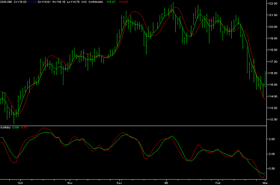
Now that we see that a prediction can be created for a theoretical waveform, and the impact of the power normalization, we can apply the LMS Predictor to real price waveforms to assess its usefulness as a technical indicator. Figure 4 shows both the Slow Stochastic predictions in the subgraph below the price bars and the Zero Lag Kalman Filter predictions overlaid on the price bars. Only the two bar prediction is displayed for clarity. Even the most cursory examination shows that both indicators have immense benefit. The Stochastic has a true predictor while the Zero Lag Moving Average lead the prediction sufficiently to used as a short term counter trender.

Figure 4.  LMS Predictions of the Slow Stochastic and Zero Lag Kalman Filter

Starting with the Stochastic and its prediction, the first buy signal occurs near the first of October and the good long position is held until the third week of October. There is a clear short signal in the fourth week of October after a little chop, going long again near the first of November. Several choppy signals ensue during November until the good long signal is given in its fourth week. Extraordinarily good signals, both long and short, are given during the months of December and January. The signals again become erratic when the cyclic swings of the Stochastic in the last week of January and the first half of February. The one very bad signal for a long entry occurs in the third week of February when the market decline continues.

Similar, but different signals are given by predicting the zero lag moving average and using the line crossings as counter trend signals. From the left of the chart, the initial good long signal is followed by an incorrect short signal in the second week of October. The long signals at the first of November and last of November turn out to be good ones. Further, every signal across the rest of the chart produce profitable results (depending on fills during those times when the cycle swings were low in amplitude).

These examples demonstrate that the LMS predictor has value in technical analysis.

CONCLUSIONS

A Least Mean Squares Predictive Filter has been described and EasyLanguage code is given to generate the prediction for both an oscillator and a zero lag Kalman filter. The benefits of the prediction as a technical analysis tool was described in terms of both theoretical waveforms and actual data examples. Next to reading tomorrows newspaper, predicting future action using advanced signal analysis techniques is perhaps the best way to peek into the future.