| CATEGORII DOCUMENTE |
| Bulgara | Ceha slovaca | Croata | Engleza | Estona | Finlandeza | Franceza |
| Germana | Italiana | Letona | Lituaniana | Maghiara | Olandeza | Poloneza |
| Sarba | Slovena | Spaniola | Suedeza | Turca | Ucraineana |
Axial deformation has been experimentally introduced in Lecture 2, when the tension test of a structural steel specimen was described. The case in point of this lecture is a systematic description of all aspects pertinent to axial deformation.
Basic Theory of Axial Deformation
The three aspects discussed
during Lecture 2, equilibrium equations, strain-displacement equations and the
constitutive relation, are applied to the case of axial deformation. A local
coordinate system ![]() , having
, having ![]() axis coincident with the longitudinal axis of the member, is
employed.
axis coincident with the longitudinal axis of the member, is
employed.
1.1 Strain-Displacement Equation
A direct consequence of part (b)
of the definition 1 is the fact that axial deformation depends only on the
variable![]() , which represents the position of a particular cross-section
on the longitudinal axis of the member.
, which represents the position of a particular cross-section
on the longitudinal axis of the member.
The physical phenomenon described by definition 1 is illustrated in Figure 1, where the undeformed and deformed conditions of the linear member are presented.
Adjacent cross-sections![]() and
and![]() originally located at distance
originally located at distance ![]() from each other, as
shown in Figure 1.a, are found after the deformation to be located at distance
from each other, as
shown in Figure 1.a, are found after the deformation to be located at distance![]() . The change in the position of the two cross-sections are described
by their displacements
. The change in the position of the two cross-sections are described
by their displacements ![]() and
and![]() , respectively.
, respectively.
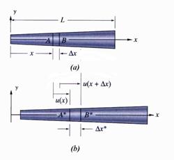
Figure 1 Geometrical Aspects of the Axial Deformation
(a) Undeformed Member and (b) Deformed Member
The extensional strain![]() is expressed as:
is expressed as:
![]() (1)
(1)
Equation (1) is called the strain-displacement equation. The cross-section
distribution of the elongation strain ![]() is shown in Figure 2. The
elongation strain is a function only of the cross-section position described by
the variable
is shown in Figure 2. The
elongation strain is a function only of the cross-section position described by
the variable![]() .
.
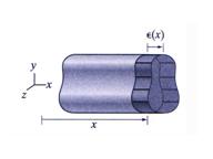
Figure 2 Extensional Strain Distribution
The rest of the generalized strain tensor components are:
![]() (2)
(2)
![]() (3)
(3)
![]() (4)
(4)
From equations (2) through (4) is evident that a transversal reduction of the cross-section takes place concomitant with the axial deformation.
The displacement ![]() pertinent to a particular cross-section is obtained by
integration from the equation (1):
pertinent to a particular cross-section is obtained by
integration from the equation (1):
![]() (5)
(5)
where ![]() is the displacement at the beginning at the integration
interval.
is the displacement at the beginning at the integration
interval.
Consequently, the total elongation of the member is calculated from equation (5) as:
![]() (6)
(6)
where ![]() is the total length of the bar.
is the total length of the bar.
Constitutive Equation
The constitutive equation
reflects, as was describe in Lecture 2, the relation between the stress and the
strain. If the linear elastic material behavior
is considered, the relation between the normal stress and extension strain ![]() for the case of the
axial deformation is written:
for the case of the
axial deformation is written:
![]() (7)
(7)
Equation (7) represents the
application of Hooks Law for the case of axial deformation. The material
constant![]() , the modulus of elasticity, has a value unique to each
specific material and is obtained from tensile tests. The cross-section of the
bar is a small surface and the variation of the modulus of elasticity is
negligible on this surface. In this case the constitutive equation (7) is
expressed as:
, the modulus of elasticity, has a value unique to each
specific material and is obtained from tensile tests. The cross-section of the
bar is a small surface and the variation of the modulus of elasticity is
negligible on this surface. In this case the constitutive equation (7) is
expressed as:
![]() (8)
(8)
Equation (8) implies that the
normal stress ![]() varies only along the
length of the member, but has a constant value on the entire cross-section. The
representation of the normal stress
varies only along the
length of the member, but has a constant value on the entire cross-section. The
representation of the normal stress ![]() is shown in Figure 3.
is shown in Figure 3.
The rest of the stress tensor components are zero:
![]() (9)
(9)
![]() (10)
(10)
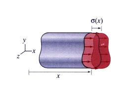
Figure 3
Cross-Section
Cross-Section Stress Resultants
Considering the stress distribution represented by equation (8) through (10) the cross-section stress resultants are obtained as:
![]() (11)
(11)
![]() (12)
(12)
![]() (13)
(13)
The relation between the normal
stress ![]() and the cross-section resultants
and the cross-section resultants![]() ,
, ![]() and
and ![]() is derived using the
notation shown in Figure 4.
is derived using the
notation shown in Figure 4.
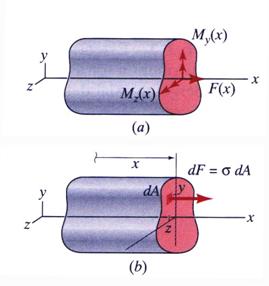
Figure 4
(a) Stress Resultants and (b) Normal Stress
If the axes ![]() and
and ![]() of the coordinate system intersect such that the
of the coordinate system intersect such that the ![]() axis passes through the cross-section centroid, the static
moments
axis passes through the cross-section centroid, the static
moments ![]() and
and ![]() are zero and the axial
force
are zero and the axial
force![]() remains the only non-zero stress resultant. Then, from
equation (11) the normal stress
remains the only non-zero stress resultant. Then, from
equation (11) the normal stress![]() is calculated as:
is calculated as:
![]() (14)
(14)
Consequently, it is to be concluded that a beam made from a linear elastic material undergoes an axial deformation if the axial force passes through the cross-section centroid.
Equilibrium Equation
The equilibrium equation pertinent
to the case of axial deformation was derived in Section 4.3 of Lecture 4. The
detailed derivation is not repeated and only the final result expressed as the
differential relation (4.7) is employed. Considering the exterior loading and stress
resultants shown in Figure 5, acting on an infinitesimal volume of length ![]() separated from the body
of the beam, the following differential equation is written:
separated from the body
of the beam, the following differential equation is written:
![]() (13)
(13)
where ![]() is the distributed
loading parallel to the beam longitudinal axis.
is the distributed
loading parallel to the beam longitudinal axis.
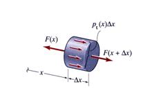
Figure 5 Infinitesimal Volume Equilibrium
If the axial stress resultant ![]() is orientated as shown in Figure 5 and tends to lengthen the
segment the internal force is called tension.
The corresponding normal stress
is orientated as shown in Figure 5 and tends to lengthen the
segment the internal force is called tension.
The corresponding normal stress ![]() is called tension stress. In contrast, if the
stress resultant force
is called tension stress. In contrast, if the
stress resultant force ![]() is orientated to shorten or compress the segment the
corresponding internal force and normal stress are called compression and compression
stress, respectively.
is orientated to shorten or compress the segment the
corresponding internal force and normal stress are called compression and compression
stress, respectively.
Integrating equation (15) the stress
resultant force ![]() is calculated:
is calculated:
![]() (16)
(16)
where ![]() is the value of the axial force at the origin of the
integration interval.
is the value of the axial force at the origin of the
integration interval.
1.5 Thermal Effects on Axial Deformation
The equations obtained in the previous sections are derived considering only the exterior load action and neglecting the change in temperature. In this section the effects of the thermal change are introduced.
During Lecture 2, the thermal
strain along the axis ![]() was introduced as:
was introduced as:
![]() (17)
(17)
where ![]() is the thermal
expansion coefficient and
is the thermal
expansion coefficient and ![]() is the change in the
member temperature.
is the change in the
member temperature.
The total elongation strain is the sum of the elongation strain induced by the exterior load action and thermal effects and is expressed as:
![]() (18)
(18)
By substitution of equation (14) into (18) the elongation strain is obtained as:
![]() (19)
(19)
Then, using equation (19) in equation (6) the total elongation of the member is written as:
![]() (20)
(20)
2 Uniform-Axial Deformation
A special case of axial deformation frequently encountered in structural engineering is the case of uniform-axial deformation shown in Figure 6. Systems composed of many members subjected to uniform-axial deformation are also commonly used in structural practice. A typical example is the plane truss, where each individual member is subjected to uniform-axial deformation under the action of to tension or compression forces.
The formulation related with the definition of the uniform-axial member and its application in the investigation of the statically determinate and indeterminate structures is presented in this section.
2.1 Members Subjected to Uniform-Axial Deformation
Definition 2 is mathematically transcribed as:
![]() (21)
(21)
![]() (22)
(22)
![]() (23)
(23)
.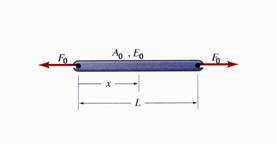
Figure 6 Member Exhibiting Uniform Axial-Deformation
Note: Equation (23) implies the absence of the distributed load ![]() in equation (15)
in equation (15)
Rewriting equations (6), (8) and (14) obtained in the previous section for the case in point of a member with uniform axial-deformation the following equations are obtained:
![]() (24)
(24)
![]() (25)
(25)
![]() (26)
(26)
In the computer applications equation (26) takes the following form:
![]() (27)
(27)
where ![]() is called the axial
stiffness coefficient.
is called the axial
stiffness coefficient.
The axial stiffness coefficient represents the force applied to the member ends when the elongation is equal with the unit length. The unit is [F/L]. The reciprocal value of the axial stiffness is called the axial flexibility coefficient. The flexibility coefficient is calculated:
![]() (28)
(28)
Using the flexibility coefficient expression equation (28) is cast in a new format:
![]() (29)
(29)
If the change in temperature is also constant along the entire length of the member the formula (20) are amended as follows:
![]() (30)
(30)
Using the flexibility coefficient
![]() the elongation is
calculated as:
the elongation is
calculated as:
![]() (31)
(31)
Rewriting the equation (31) the
force ![]() is obtained:
is obtained:
![]() (32)
(32)
Statically Determinate Structure
An example of a statically
determinate structure is shown in Figure 7. A rigid, weightless beam AC is
supported at end A by a column and at end C by a vertical rod CD. The rod is
attached at point D to a leveling jack, a component which permits a limited
vertical movement and has the mission to keep the beam AC leveled. The beam AC
is loaded with a vertical force P located at distance ![]() from the left end A.
To calculate the axial forces acting on the column and rod the system is
decomposed into three components: the beam, the column and the rod.
from the left end A.
To calculate the axial forces acting on the column and rod the system is
decomposed into three components: the beam, the column and the rod.
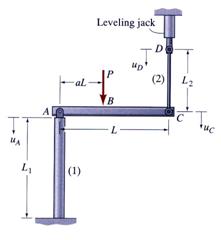
Figure 7 Statically Determinate Structure
The free-body diagram of the beam
is depicted in Figure 8 and is used to calculate the reaction forces ![]() and
and![]() . The connection between the column and the beam requires in
general, two reaction forces. In the absence of any horizontal force the
horizontal component is null and is not shown
. The connection between the column and the beam requires in
general, two reaction forces. In the absence of any horizontal force the
horizontal component is null and is not shown
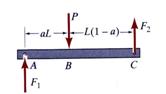
Figure 8 Free-Body Diagram
The reaction forces can be calculated using the following equilibrium equations:
![]()
![]() (33)
(33)
![]()
![]() (34)
(34)
Solving equations (33) and (34) the reaction forces are obtained:
![]() Compression in column (35)
Compression in column (35)
![]() Tension in rod (36)
Tension in rod (36)
Note: The column and the rod are loaded with forces having opposite directions than the reaction forces calculated in equations (35) and (36). This became obvious if one attempt to draw the free-body diagram for the rod and column.
From equations (35) and (36) it
is evident that the column and the rod are loaded with compression force ![]() and tension force
and tension force ![]() , respectively. These two elements are characterized, using
definition 2, as members with uniform axial-deformation.
, respectively. These two elements are characterized, using
definition 2, as members with uniform axial-deformation.
Using the formulae (24) through (26) the following related column values are calculated:
![]() (37)
(37)
![]() (38)
(38)
![]() (39)
(39)
Note: The force ![]() is compression and the
column is shortened by the loading action.
is compression and the
column is shortened by the loading action.
Related quantities for the rod CD are similarly calculated:
 (40)
(40)
![]() (41)
(41)
![]() (42)
(42)
Note: The force ![]() is tension and the rod
is elongated by the loading action.
is tension and the rod
is elongated by the loading action.
For the beam to stay in perfect horizontal balance the displacement at point A and C should be equal and manifest in the same direction:
![]() (41)
(41)
The expressions of the displacements at points A and C are calculated using the formula (5).The displacement at point A is equal with the column elongation, because the initial displacement at ground connecting point is considered zero:
![]() (42)
(42)
The displacement at point C is calculated as:
![]() (43)
(43)
where ![]() is the displacement
allowed by the leveling jack.
is the displacement
allowed by the leveling jack.
The necessary displacement allowed by the leveling device is calculated from equation (41):
 (44)
(44)
Note: The displacement ![]() has to be positive for
the device to work properly (the device works only in tension). This means that
the deformation of the column has to be larger than the rod deformation.
has to be positive for
the device to work properly (the device works only in tension). This means that
the deformation of the column has to be larger than the rod deformation.
The numerical application for this example is presented in section 6.1.
Statically Indeterminate Structure
A typical example of a statically indeterminate structure is shown in Figure 9. This type of structures requires a more involved methodology for in order to calculate the stress and strain distributions.
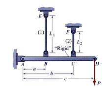
Figure 9 Statically Indeterminate Structure
The system shown in Figure 9 is
composed of a rigid member AD, pinned into the wall at point A, and two unequal
linear elastic rods, BE and CF. The rods, BE and CF, are attached to the
ceiling at points E and F, respectively. The system is loaded with a
concentrated vertical force ![]() at point D. The
free-body diagram used to write the equilibrium equations is shown in Figure 10.
at point D. The
free-body diagram used to write the equilibrium equations is shown in Figure 10.
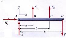
Figure 10 Free-Body Diagram
The following equilibrium equations are written:
![]()
![]() (47)
(47)
![]()
![]() (48)
(48)
![]()
![]() (49)
(49)
The equilibrium equations (48)
and (49) contain three unknown reaction forces![]() ,
, ![]() and
and ![]() . In order to solve these unknown quantities one additional
equation is necessary. This equation is obtained from the deformation
compatibility condition schematically described in Figure 11. Because the beam
AD is rigid, purely geometric relations between the rod elongations,
. In order to solve these unknown quantities one additional
equation is necessary. This equation is obtained from the deformation
compatibility condition schematically described in Figure 11. Because the beam
AD is rigid, purely geometric relations between the rod elongations,![]() and
and![]() , and the rotation angle
, and the rotation angle ![]() are written as:
are written as:
![]() (50)
(50)
![]() (51)
(51)
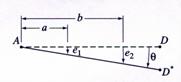
Figure 11 Deformation Notation
Using equation (29) and the relations (50) and (51) the forces in the rods are expressed as:
![]() (52)
(52)
![]() (53)
(53)
The stiffness coefficients, ![]() and
and![]() , are calculated from the geometrical and material properties
characteristics of the rods:
, are calculated from the geometrical and material properties
characteristics of the rods:
![]() (54)
(54)
![]() (55)
(55)
Substituting equations (52) and (53)
into the equilibrium equations (48) and (49),![]() and
and ![]() are eliminated from
the system leaving only two unknowns,
are eliminated from
the system leaving only two unknowns, ![]() and
and![]() :
:
![]() (56)
(56)
![]() (57)
(57)
Solving the algebraic system, the two unknowns are found as:
![]() (58)
(58)
where ![]() is the rotation angle
corresponding to
is the rotation angle
corresponding to ![]()
 (59)
(59)
Introducing the rotation angle ![]() into equations (52)
and (53) the rod forces are calculated:
into equations (52)
and (53) the rod forces are calculated:
![]() (60)
(60)
![]() (61)
(61)
where ![]() and
and ![]() are the forces in the
rods in
are the forces in the
rods in ![]()
The rod stresses are also calculated:
![]() (62)
(62)
![]() (63)
(63)
The rod elongations are obtained using equations (50) and (51) as:
![]() (64)
(64)
![]() (65)
(65)
If the allowable vertical force ![]() is required, the
stress in the rods must be compared against the allowable stress
is required, the
stress in the rods must be compared against the allowable stress![]() :
:
![]() (66)
(66)
 (67)
(67)
At limit, the relations (66) and (67) are rewritten as:
![]() (68)
(68)
![]() (69)
(69)
Introducing the rod forces, equations (60) and (61), into equations (68) and (69) the allowable vertical force admitted by the system is calculated as:
 (70)
(70)
The numerical application for this example is presented in section 6.2.
3 Nonuniform-Axial Deformation
The definition of a member with uniform-axial deformation is specified in Section 3. If any one of the assumptions contained in definition 2 is violated the axial deformation is called nonuniform-axial deformation. The most common cases of nonuniform-axial deformation are treated in the following subsections.
Non-homogeneous Cross-Section Members
The theory developed in the previous sections assumed that the cross-section is made from a homogeneous material described by its modulus of elasticity. In structural engineering practice it is not uncommon to have a case in which a member constructed from two different materials bounded together at their interface is forced to undergo an axial deformation. The members made from different materials but behaving together as a single member are called composite sections.
For the purpose of analysis it is
assumed that the member is made from two materials, each being characterized by
a specific modulus of elasticity (![]() and
and![]() ) and area (
) and area (![]() and
and![]() ). The strain distribution is, as before, assumed to be a
function of only the variable
). The strain distribution is, as before, assumed to be a
function of only the variable![]() , the position of the particular cross-section of interest:
, the position of the particular cross-section of interest:
![]() (71)
(71)
Considering that both materials are homogeneous linear elastic materials the Hooks law may be written for each material as:
![]() (72)
(72)
![]() (73)
(73)
The total axial force ![]() , as expressed in equations (11), is divided into two axial
forces, each acting at the centroid of the corresponding bar cross-section.
, as expressed in equations (11), is divided into two axial
forces, each acting at the centroid of the corresponding bar cross-section.
 (74)
(74)
where
![]() (75)
(75)
![]() (76)
(76)
Substituting the axial stresses expressed in equations (72) and (73) into equations (75) and (76) the equilibrium equation (74) is written as:
 (77)
(77)
Consequently, the elongation strain is obtained:
![]() (78)
(78)
Accordingly, the normal stresses are calculated employing the equations (72) and (73) as:
![]() (79)
(79)
![]() (80)
(80)
In general, the stress resultant moments, as expressed in equations (12) and (13), do not vanish and additional restrictions regarding the geometrical characteristics of the cross-section must be imposed. Nullification of the stress resultant moments is obtained by using symmetric cross-section about one or both centroidal axes.
The frequently encountered
practical case when the areas ![]() and
and![]() are constants along the entire length and the member is
subjected to a constant force
are constants along the entire length and the member is
subjected to a constant force ![]() is considered below.
It is additionally assumed that the cross-section is symmetrical only about the
vertical axis
is considered below.
It is additionally assumed that the cross-section is symmetrical only about the
vertical axis ![]() . Then, the normal stresses developed in each material zone
are calculated, following the equations (79) and (80), as:
. Then, the normal stresses developed in each material zone
are calculated, following the equations (79) and (80), as:
![]() (81)
(81)
![]() (82)
(82)
The assumption regarding the
symmetrical aspect of the cross-section about the vertical axis nullify the
stress resultant moment ![]() when the bar local
coordinate system is centroidal. The second stress resultant moment
when the bar local
coordinate system is centroidal. The second stress resultant moment ![]() can be made zero by
manipulating the position of the application of the force
can be made zero by
manipulating the position of the application of the force ![]() . It was previously argued that the individual cross-section
resultants
. It was previously argued that the individual cross-section
resultants ![]() and
and ![]() must be located at the centroids of the cross-sections
must be located at the centroids of the cross-sections![]() and
and![]() . This raises the question about the location of the applied force
. This raises the question about the location of the applied force![]() in order that only axial forces are induced in each of the
individual bars composing the cross-section. This situation is solved by
replacing the axial forces
in order that only axial forces are induced in each of the
individual bars composing the cross-section. This situation is solved by
replacing the axial forces ![]() and
and ![]() with a resultant force
and a null moment written about a horizontal axis. The stress resultant moment about the vertical
axis has a zero value due to the imposed symmetry of the cross-section about
that axis. The moment equation, written about an horizontal axis passing
through the application point of the force
with a resultant force
and a null moment written about a horizontal axis. The stress resultant moment about the vertical
axis has a zero value due to the imposed symmetry of the cross-section about
that axis. The moment equation, written about an horizontal axis passing
through the application point of the force ![]() , is:
, is:
![]() (83)
(83)
where ![]() is the distance
between the centroids of cross-sections
is the distance
between the centroids of cross-sections![]() and
and![]() , while
, while ![]() is the distance
between the application point of the force
is the distance
between the application point of the force ![]() and the centroid of
the area
and the centroid of
the area ![]() .
.
The distance ![]() is then calculated:
is then calculated:
![]() (84)
(84)
Note: In general the application point of the force ![]() does not correspond
with the centroid of the composite cross-section.
does not correspond
with the centroid of the composite cross-section.
3.2 Non-homogeneous Cross-Section Members Subjected to Thermal Changes
Consider the composite section
described in Section 3.1 subjected to change in temperature. For generality, in
this discussion, let be assumed that each individual bar undergoes a different
change in temperature ![]() and
and![]() , respectively. The notation employed in the Section 3.1 is
maintained. In the absence of the exterior forces, the equation of equilibrium
is:
, respectively. The notation employed in the Section 3.1 is
maintained. In the absence of the exterior forces, the equation of equilibrium
is:
![]() (85)
(85)
The axial forces pertinent to each one of the bars is constant along their respective lengths and thus, the equation (85) becomes:
![]() (86)
(86)
The equilibrium equation contains
two unknown cross-sectional forces,![]() and
and ![]() , and consequently the system is statically indeterminate. An
additional equation is necessary to obtain these forces. This equation is derived
from the condition of equality of the elongations for the two individual bars
imposed by the existence of the rigid members attached at their ends. This
equation is written as:
, and consequently the system is statically indeterminate. An
additional equation is necessary to obtain these forces. This equation is derived
from the condition of equality of the elongations for the two individual bars
imposed by the existence of the rigid members attached at their ends. This
equation is written as:
![]() (87)
(87)
The elongations may be express using the formulation of equation (31):
![]() (88)
(88)
![]() (89)
(89)
Substituting equations (88) and (89) into equation (87) the second necessary equation is obtained:
![]() (90)
(90)
Solving the algebraic equation system (86) and (90) the cross-section forces are calculated:
![]() (91)
(91)
The axial stress in the bars is:
![]() (92)
(92)
![]() (93)
(93)
3.3 Heated Member with a Linear Temperature Variation
The slender beam shown in Figure 12.a
is heated by a heating coil capable of producing a linearly varying temperature
as shown in Figure 12.b. The beam has a constant cross-section area ![]() and is made from a linear elastic material. The beam is
attached to rigid supports at ends A and B.
and is made from a linear elastic material. The beam is
attached to rigid supports at ends A and B.
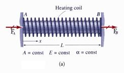
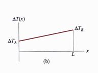
Figure 12 Heated Uniform Member
(a) Geometry and (b) Temperature Variation
In the absence of any applied forces between A and B, the equilibrium equation is written as:
![]() (94)
(94)
The system is statically
indeterminate containing two unknown reaction forces ![]() and
and![]() . An additional equation is necessary. This equation is
obtained by observing that the total elongation of the beam is null:
. An additional equation is necessary. This equation is
obtained by observing that the total elongation of the beam is null:
![]() (95)
(95)
Following the equations (20) and (31) the total elongation is calculated:
![]() (96)
(96)
where ![]()
Accordingly, with the temperature variation shown in Figure 12.b the thermal variation in a particular cross-section is:
![]() (97)
(97)
The integral contained in the equation (96) is calculated using the expression (97):
 (98)
(98)
Substituting (98) into (96) the total elongation is expressed as:
![]() (99)
(99)
Imposing the condition (95) the
force ![]() is found:
is found:
 (100)
(100)
Using the equation (94) results that:
![]() (101)
(101)
The normal stress is then calculated as:
![]() (102)
(102)
4 Special Aspects
4.1 Normal Stress in the Vicinity of the Load Application
A vertical prismatic bar
characterized by a constant cross-section along its entire length![]() is loaded at one end by a concentrated force
is loaded at one end by a concentrated force![]() and supported at the other end as illustrated in Figure 13.
Based on
and supported at the other end as illustrated in Figure 13.
Based on ![]() opposed to the action.
The free-body diagram is shown in Figure 13.a. The example considered falls in
the category of members with uniform axial-deformation studied in Section 2.
The exact determination of the distribution of normal stress along the length
of the beam requires advanced methodologies employed in the Theory of
Elasticity and for this reason only the results are presented. Analyzing the
results illustrated in Figure 13 it is found that the formulae obtained in Section
2 are valid in the majority of the cross-sections except of those located in
the vicinity of the ends. The perturbation zone has a length
opposed to the action.
The free-body diagram is shown in Figure 13.a. The example considered falls in
the category of members with uniform axial-deformation studied in Section 2.
The exact determination of the distribution of normal stress along the length
of the beam requires advanced methodologies employed in the Theory of
Elasticity and for this reason only the results are presented. Analyzing the
results illustrated in Figure 13 it is found that the formulae obtained in Section
2 are valid in the majority of the cross-sections except of those located in
the vicinity of the ends. The perturbation zone has a length ![]() roughly equal to the width of the cross-section.
roughly equal to the width of the cross-section.
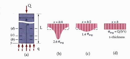
Figure 13
Note: It can be concluded that for practical purposes the formulae
obtained in Section 2 based on the assumptions contained in definition 1 are
valid especially if the ratio![]() . Special attention has to be given to the areas located near
the point of load application or near abrupt changes in the cross-section. The
application of Saint Venants Principle is valid for the case of the beam.
. Special attention has to be given to the areas located near
the point of load application or near abrupt changes in the cross-section. The
application of Saint Venants Principle is valid for the case of the beam.
4.2 Stress Concentrations
In the theoretical development
pertinent to the axial deformation of linear members, the area ![]() of the cross-section is considered as a smoothly varying
function of the position
of the cross-section is considered as a smoothly varying
function of the position ![]() . If discontinuities appear in the definition of the
cross-sectional area, the formulae obtained in the preceding sections are
invalid and the concept of stress
concentration must be introduced.
. If discontinuities appear in the definition of the
cross-sectional area, the formulae obtained in the preceding sections are
invalid and the concept of stress
concentration must be introduced.
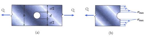
Figure 14 Concentration of Stress
A typical case is shown in Figure
14 where a prismatic type linear member having a circular hole of diameter ![]() is subjected to a
constant tension force
is subjected to a
constant tension force![]() . The member cross-section is described by the height
. The member cross-section is described by the height ![]() and thickness
and thickness![]() .
.
The normal stress ![]() around the hole can be significantly greater than
around the hole can be significantly greater than ![]() and varies as a function
of the ratio
and varies as a function
of the ratio![]() . For practical applications the coefficient
. For practical applications the coefficient![]() , called the stress-concentration
factor is introduced. This factor is
defined as the ratio of the maximum normal stress
, called the stress-concentration
factor is introduced. This factor is
defined as the ratio of the maximum normal stress ![]() around the hole to the normal stress calculated in the
absence of the hole
around the hole to the normal stress calculated in the
absence of the hole![]() , called nominal
stress.
, called nominal
stress.
![]() (103)
(103)
![]() . (104)
. (104)
The average normal stress calculated with the formula (14) is:
![]() . (105)
. (105)
The variation of the
stress-concentration factor ![]() , calculated using the Theory of Elasticity methods is
illustrated in Figure 1 The stress concentration factor for the configuration
under consideration varies from 2.3 to 3.0.
, calculated using the Theory of Elasticity methods is
illustrated in Figure 1 The stress concentration factor for the configuration
under consideration varies from 2.3 to 3.0.
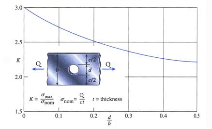
Figure 15 Variation of the Stress-Concentration Factor
Analyzing the variation, it is
concluded that if the diameter![]() decreases the concentration factor
decreases the concentration factor ![]() also increases. This is somewhat misleading and is due to the
way the chart in Figure 15 is constructed. Using the average normal stress
also increases. This is somewhat misleading and is due to the
way the chart in Figure 15 is constructed. Using the average normal stress![]() in the definition of the stress concentration factor
in the definition of the stress concentration factor![]() , equation (103) the following formula is obtained:
, equation (103) the following formula is obtained:
![]() (106)
(106)
Considering the extreme cases
shown in Figure 15 and applying these within equation (106) it can be concluded
that the maximum normal stress ![]() increases with the increase in the diameter of the hole and
varies as:
increases with the increase in the diameter of the hole and
varies as:
![]() (107)
(107)
For small diameter holes the stress concentration disappears at relatively small distance from the hole. This is an example of the application of Saint Venants Principle.
4.3 Limits of Poissons Ratio
The volumetric strain![]() was calculated in Section 2.9.3 for the general case when the
normal stresses
was calculated in Section 2.9.3 for the general case when the
normal stresses![]() ,
, ![]() and
and ![]() are applied simultaneously. For the case of axial deformation
only the normal stress
are applied simultaneously. For the case of axial deformation
only the normal stress ![]() has a non-zero value
and, consequently, the equation (2.111) is written as:
has a non-zero value
and, consequently, the equation (2.111) is written as:
![]() (108)
(108)
Because the volume can not decrease during the tensioning of the axially deformed member the volumetric strain is a positive value. Mathematically this condition is enforced as:
![]() (109)
(109)
Consequently, from physical reality and equation (108) it is seen that:
![]() (110)
(110)
The limits established for Poissons ratio ![]() by the expression (110)
are generally valid for all materials used in structural engineering. The cases
representing the limiting values,
by the expression (110)
are generally valid for all materials used in structural engineering. The cases
representing the limiting values, ![]() and
and ![]() , are pertinent to cork and water, respectively. Structural
steel has a Poissons ratio of 0.33. There are some cases when the material has
a negative Poissons ratio. These materials are called swollen solids and this unusual behavior is characteristic of certain
materials subjected to radiation.
, are pertinent to cork and water, respectively. Structural
steel has a Poissons ratio of 0.33. There are some cases when the material has
a negative Poissons ratio. These materials are called swollen solids and this unusual behavior is characteristic of certain
materials subjected to radiation.
The transversal contraction of the cross-section is similarly obtained as:
![]() (111)
(111)
5 Design of Members Subjected to Axial Deformation
In the design of the members
subjected to axial deformation two important factors, the load ![]() and the resistance
and the resistance ![]() , are considered. The load
, are considered. The load ![]() represents the maximum
axial force that occurs in the specific member when subjected to the action of
exterior forces or change in temperature. The most common definition for the resistance
represents the maximum
axial force that occurs in the specific member when subjected to the action of
exterior forces or change in temperature. The most common definition for the resistance
![]() is the force which is
developed in the member when the normal stress reaches the yielding value
is the force which is
developed in the member when the normal stress reaches the yielding value![]() .
.
The design of the member
subjected to axial deformation is conducted under the condition that the
capacity of the member, represented by its resistance force![]() , must always be greater or equal to the demand force
, must always be greater or equal to the demand force ![]() . Mathematically, this assumption is expressed as:
. Mathematically, this assumption is expressed as:
![]() (112)
(112)
In the calculation of the load ![]() and resistance
and resistance ![]() forces there are
typically a number of factors (load magnitudes and directions, material
characterization, manufacturing tolerance, etc.) which are not known with
absolute certainty. The degree of uncertainty may be treated using the concepts
proper of Probability Theory. In order to circumvent the difficulties inherent
in the rigorous application of probabilistic methods, a global factor
forces there are
typically a number of factors (load magnitudes and directions, material
characterization, manufacturing tolerance, etc.) which are not known with
absolute certainty. The degree of uncertainty may be treated using the concepts
proper of Probability Theory. In order to circumvent the difficulties inherent
in the rigorous application of probabilistic methods, a global factor ![]() , called the safety
factor, encompassing all possible uncertainties is introduced as:
, called the safety
factor, encompassing all possible uncertainties is introduced as:
![]() (113)
(113)
The allowable resistance ![]() is then used in place
of the resistance
is then used in place
of the resistance ![]() in equation (112).
in equation (112).
![]() (114)
(114)
The safety factor is always greater than or equal to unity:
![]() (115)
(115)
This is the approach used by the method called ultimate strength design method and was adopted by American Concrete Institute (ACI) and American Institute of Steel Construction (AISC).
If the relation between the stress and strain is linear, than a similar safety factor may be defined by limiting the value of the normal stress in the axially deformed member.
![]() (116)
(116)
The design formula (114) is modified
using the relationship between maximum normal stress ![]() and the allowable normal
stress
and the allowable normal
stress![]() :
:
![]() (117)
(117)
The formula (117) was used for a
long period of time in a procedure known as the allowable-stress design. Due to the simplicity of application, this
method is still commonly used in
6 Examples
The application of the theoretical formulae developed in this lecture is illustrated in the following examples.
Statically Determinate Structure
The structure illustrated in Figure 7 was investigated in Section 2. The following numerical values are considered in the numerical application of the generic formulation:
![]()
![]()
![]()
![]()
![]()
![]()
![]()
![]()
![]()
![]()
![]()
![]()
![]()
![]()
![]()
![]()
![]()
The reaction forces are:
![]()
![]() Compression in column
Compression in column
![]()
![]() Tension in rod
Tension in rod
The column related values are:
![]()
![]()
![]()
![]()
![]()
The rod related values are:
![]()
![]()
![]()
![]()
![]()
The displacement ![]() of the leveling device
is calculated as:
of the leveling device
is calculated as:
![]()
![]()
Statically Indeterminate Structure
The statically indeterminate structure illustrated in Figure 9 is solved in Section 2.3. For the numerical application of the formulation developed the following data are employed:
![]()
![]()
![]()
![]()
![]()
![]()
![]()
![]()
![]()
![]()
![]()
![]()
![]()
![]()
![]()
![]()
![]()
![]()
The stiffness coefficients are:
![]()
![]()
![]()
![]()
The rotation angle ![]() is:
is:
![]()
![]()
The rod forces ![]() and
and ![]() are calculated as:
are calculated as:
![]()
![]()
![]()
![]()
The allowable vertical force ![]() for the system is:
for the system is:
![]()
![]()
|
Politica de confidentialitate | Termeni si conditii de utilizare |

Vizualizari: 5987
Importanta: ![]()
Termeni si conditii de utilizare | Contact
© SCRIGROUP 2026 . All rights reserved