| CATEGORII DOCUMENTE |
| Asp | Autocad | C | Dot net | Excel | Fox pro | Html | Java |
| Linux | Mathcad | Photoshop | Php | Sql | Visual studio | Windows | Xml |
There is also a host of financial functions available in Excel. The ones you choose to use will depend upon your job function. If, for example, you are a financial analyst, you might use IRR to calculate the internal rate of return on an investment. If you work in finance, you may a need DB to calculate the declining balance of an asset, or DDB to calculate the double declining balance. What these functions have in common is that most of them relate to the term of an investment, the flow of payments, the rate of interest or discount, and the amount of the payment.
In this section, we will focus on three financial functions: PV, FV, and PMT.
PV is used to calculate the present value of a series of payments. FV is used to calculate the future value of a series of payments, and the PMT function is used to calculate the amount of a payment over time. These functions are used in banking and investment all the time.
PMT (payment)
Let's assume you have loaned me $5,000. We then agree that I will send you a payment once a month for two years. The simple interest rate on this loan is 12 percent. Each month for two years, you'll receive a payment, part of which represents principal and part of which is interest. In other words, an additional 12 percent is paid to you as compensation for the risk you have assumed (I might not pay you back).
How much do I owe you on the first of each month? To calculate this amount, we use the PMT function of Excel. In order to use the PMT function, we need to know three things: the interest rate, the number of payments, and the principal amount of the loan.
Look at the setup on Sheet 9 in your workbook for this lesson and you'll see how this example is constructed. Note that in cell A4, we want to calculate the payment. Here's the PMT function we used to get the payment amount:
=PMT(B2/12,B3,B1)*-1When dealing with an interest rate that is quoted as an annual percentage but your term is quoted in months, you have to convert the annual percentage to monthly interest. This is done in our example by dividing the contents of cell B2 by 12. Generally the PMT formula will output a negative number because payments reduce the amount owed. In this example, we have multiplied by -1 to display this as a positive number.
If your periods are shown in years but the payments should occur monthly, you have to multiply the number of periods by 12 to get the total number of actual monthly payments being made. In our example, we have 24 months as the term, so we didn't have to multiply by 12 to get the total number of monthly payments.
the Insert/Function
It's impossible to carry around in your head the requirements of all the functions you will use in Excel. This is why Excel provides the Insert/Function sequence of dialog boxes. They are accessed from the Insert menu and display the following logically grouped dialog boxes.

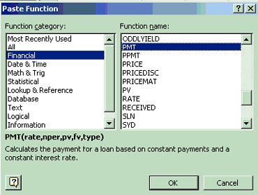
Figure 1-9: The Insert/Function dialog box
As you can see, the function categories are on the left side of the dialog box, and the categorized functions are shown in the list box on the right. To access the financial functions, click Financial in the list box. To select PMT, scroll the right-hand list box until PMT comes into view. Click it, and then click OK. The setup is shown in Figure 1-9.
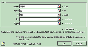
The PMT function dialog box appears next. Each function has an associated dialog box, like the one shown in Figure 1-10. For some reason, it appears directly over the area where you want to work. Consequently, you will have to click and drag it away from the cells containing the information you need in the calculation.

Figure 1-10: The PMT function dialog box.
This dialog box is used in the following way: Click in the first field requiring information (these are the fields in bold). Then click in the cell containing the relevant value. If you need to perform a calculation on the cell's value, such as the interest rate, click in that dialog field and type what's needed. You can see B2/12 in our example. Click in the next field and then click in the next required worksheet cell. Continue this process until you've filled in all required values. Finally, click OK.
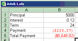
After you click the OK button, the formula will calculate and you will see your payment represented as a negative number. Again, this makes sense because a payment reduces the amount owed. However, most people prefer to see their payment as a positive number. To convert the payment amount to a positive value, you must multiply the entire formula by -1. It's fine if you want to do this on your worksheet now. Also, calculate the total of the payments in cell B5. This is simply the payment amount multiplied by the term. When complete, your worksheet looks like the sample below:

Figure 1-11: The completed worksheet
PV (present value)
Let's assume that you and I are involved in a business deal and I've agreed to pay you $500 per month for the next 24 months for a load of widgets I purchased at 12 percent interest. I decide I would rather pay you off today in full than string the payments out over the next two years. The question you must answer is how much are you willing to accept today.
If we don't settle up today, and I give you your 24 payments, you receive a total of $12,000. Remember, a dollar in hand today is worth more than a dollar in hand two years from now. You decide to accept my offer, because you think you can invest the money elsewhere and receive an even larger return. To figure out what you will accept today, we use the PV, or Present Value function.
The function takes the following arguments:
=PV(Rate, Nperiods, Payment)In our case, on Sheet 9 these values are found in cells B8, B9, and B10. Remember, we have to convert interest into a monthly interest rate by dividing by 12. Our formula for calculating PV looks like this:
=PV(B9/12,B10,B8)*-1Again, note we've multiplied by a negative one to turn the result into a positive number. We've also divided the interest rate in B9 by 12 so the function uses monthly interest rates.
On your own, using the Insert/Function dialogs, build the PV formula in cell B12 on Sheet 9 of your workbook. Your finished result should be equal to $10,621.69. Don't forget to multiply by negative one.
FV (future value)
The last financial function we cover in this lesson is FV, or Future Value. Let's assume you're in a position to save $500 each month for the next three years. You have located a nice little fund that pays 14 percent and you want to know how much your investment will be worth three years from the first month you make your deposit into the fund. To use FV, we need to know the amount of the payment, the rate of interest, and the term of the investment. Remember we are dealing here with monthly interest rates, and total payments. Our setup on sheet 9 is as follows:
Our formula for FV, or future value is shown below:
=FV(B16/12,B17,B15)*-1Go to Sheet 9 in your workbook for this lesson and use the Insert/Function dialogs to construct the FV formula. Remember to divide interest rate by 12, and multiply the final formula by a negative one.
For your trouble you've made $1,756.59. Just for fun, experiment with the FV calculation and see how much money you would have if you did this for 25 years. As you see, FV is a handy retirement planning device.
|
Politica de confidentialitate | Termeni si conditii de utilizare |

Vizualizari: 1373
Importanta: ![]()
Termeni si conditii de utilizare | Contact
© SCRIGROUP 2026 . All rights reserved