| CATEGORII DOCUMENTE |
| Asp | Autocad | C | Dot net | Excel | Fox pro | Html | Java |
| Linux | Mathcad | Photoshop | Php | Sql | Visual studio | Windows | Xml |
Color management is an essential part of the image acquisition, image processing, and image output workflow. Because most image input and output devices specify color in red/green/blue (RGB), YUV, or another device-dependent color space, the color appearance of pixels can shift when an image is moved from one device to another. Color management systems quantify these differences and then use color transformations to create device-independent colors, and also provide a mechanism for predicting how colors will appear on different devices.
The Image Processing Toolbox includes an open color management module that provides color space conversions and support for International Color Consortium (ICC) color profiles to facilitate a color-managed workflow. In this article, we use a soft-proofing example to show how these features work together.
Color is an experience. When light reflects off a colored object, the human eye senses color. Technically, the measure of the power, called the spectral power distribution (SPD), carried by each frequency or "color" in a light source (illuminant) and the colored object (colorant) combine to produce reflected light with a particular SPD. This light interacts with the three types of color-sensitive cones in the human eye to produce nerve impulses that the brain interprets as a specific color. If the SPD of either the illuminant or the colorant changes, the perceived color also is likely to change. As the SPDs and many aspects of the human visual system can be readily modeled using linear algebra, MATLAB is suited to working with spectral color.
Color is measurable. Spectrophotometers and colorimeters give descriptions of individual colors and are the basic hardware of color management. The measured values may be amounts of energy at different parts of the visible spectrum (an SPD) or they may be the intensities of light passing through colored filters or sensors. When compared with reference targets, these measurements describe the device that produced them.
Color is describable. Spectral color is useful for unambiguously describing a color, but it can be unwieldy for describing large numbers of colors. It is much more common to use a color space that translates numeric triples (and sometimes quadruples) into a specific color. In the case of RGB, these numbers are device-dependent combinations of red, green, and blue light. For color systems such as XYZ and L*a*b* these device-independent values are modeled on aspects of the human visual system. There are many other color spaces and color appearance models.
The ICC, of which The MathWorks is a member, has created a color profile specification that provides a mechanism for communicating color information among devices. An additional component, the color management module (CMM), acts on color images and profiles.
The Image Processing Toolbox provides several functions that implement a CMM, including support for reading and writing ICC profiles, creating color transformations, and applying profiles to images. You can access the code for all these functions, removing the inscrutability that is usually part of a CMS. Here, we examine an ICC profile that ships with the Image Processing Toolbox.
sRGB_profile
= iccread(
'sRGB.icm'
sRGB_profile
=
|
Header: |
[1x1 struct] |
|
TagTable: | |
|
Copyright: |
'Copyright (c) 1999 Hewlett-Packard Company' |
|
Description: |
[1x1 struct] |
|
MediaWhitePoint: | |
|
MediaBlackPoint: | |
|
DeviceMfgDesc: |
[1x1 struct] |
|
DeviceModelDesc: |
[1x1 struct] |
|
ViewingCondDesc: |
[1x1 struct] |
|
ViewingConditions: |
[1x1 struct] |
|
Luminance: | |
|
Measurement: | |
|
Technology: | |
|
MatTRC: |
[1x1 struct] |
|
PrivateTags: | |
|
Filename: |
'sRGB.icm' |
The fields in the structure contain all the fields from the ICC profile.
For example, the MediaWhitePoint field contains the XYZ color space
coordinates for the white point, while the MatTRC field is a structure of the RGB primaries (again in
XYZ) and the tone responsive curves. A TRC maps input pixel values to device
output values, and is essentially a gamma correction.
sRGB_profile.MatTRC
ans =
|
RedColorant: | |
|
GreenColorant: | |
|
BlueColorant: | |
|
RedTRC: |
[1024x1 uint16] |
|
GreenTRC: |
[1024x1 uint16] |
|
BlueTRC: |
[1024x1 uint16] |
How do we know that the values are XYZ coordinates? The Header field contains the profile
connection space (PCS):
sRGB_profile.Header
ans =
|
Size: | |
|
CMMType: |
'appl' |
|
Version: | |
|
DeviceClass: |
'display' |
|
ColorSpace: |
'RGB' |
|
ConnectionSpace: |
'XYZ' |
|
CreationDate: |
'03-Dec-1999 17:30:00' |
|
Signature: |
'acsp' |
|
PrimaryPlatform: |
'Apple' |
|
Flags: | |
|
IsEmbedded: | |
|
IsIndependent: | |
|
DeviceManufacturer: |
'IEC ' |
|
DeviceModel: |
'sRGB' |
|
Attributes: | |
|
IsTransparency: | |
|
IsMatte: | |
|
IsNegative: | |
|
BlackandWhite: | |
|
RenderingIntent: |
'perceptual' |
|
Illuminant: | |
|
Creator: |
'HP ' |
This profile is for the sRGB color space, an ISO standard color space that attempts to match the typical PC monitor. Encoding a color in a widely understood format provides a convenient way to work with device-dependent color when you don't know the characteristics of the target device.
Actually, every device in a color-managed workflow must be individually calibrated and characterized. Calibration brings a device close to an optimal state, while characterization describes the device's color settings in that state. Typically, we use a colorimeter to characterize the device and to obtain an ICC profile.
Suppose we want to soft-proof an image as it would appear printed on paper. We first load the image and associate it with a color profile. This image has been saved in the sRGB color space. We'll assume that we are going to display it on an sRGB monitor.
peppers_sRGB = imread('peppers.png'
sRGB_profile
= iccread('sRGB.icm'
figure; imshow(peppers_sRGB)
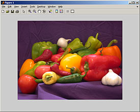
Click on image to see enlarged view.
This image contains some highly saturated colors that many printers can't reproduce. The range of colors a device or printed medium can display, or its gamut, varies from one device to another, and depends on the device's primaries and white point. For an emissive device, such as a CRT monitor, the primaries are the "pure" red, green, and blue colors. The white point is the color of the brightest neutral color on the device, or "white." For a print, the gamut depends on the output device, the paper, and the ink set.
During printing, the system must map "out-of-gamut" colors to colors the
printer can produce. In the Image Processing Toolbox, the MAKECFORM and APPLYCFORM functions perform color
space conversions and associated gamut mapping. Let's
soft-proof the image by simulating printing on an Epson Stylus Photo 2200,
using two different Epson papers. (You can download the ICC profiles for
the Epson Stylus Photo 2200 from Epson's Website.)
The ICCREAD function imports ICC
profiles. The ICCFIND and ICCROOT commands in the Image
Processing Toolbox 5.1 also help us manage and load profiles installed by the
operating system.
[profiles, names] =
iccfind(iccroot,
profiles =
[1x1
struct]
[1x1 struct]
[1x1 struct]
[1x1 struct]
[1x1 struct]
[1x1 struct]
[1x1 struct]
[1x1 struct]
[1x1 struct]
[1x1 struct]
[1x1 struct] names =
'Stylus
Photo 2200'
'Epson 2200 - Premium Luster'
'SP2200 Enhanced Matte_MK'
'SP2200 Enhanced Matte_PK'
'SP2200 Premium Glossy_PK'
'SP2200 Premium Luster_PK'
'SP2200 Premium Semigloss_PK'
'SP2200 Velvet Fine Art_MK'
'SP2200 Velvet Fine Art_PK'
'SP2200 Watercolor - RW_MK'
'SP2200 Watercolor - RW_PK'
To see how the image might look on Epson Velvet Fine Art paper with matte black ink and on Epson Premium Glossy paper with photo black ink, we enter the following commands.
glossy_profile =
profiles;
velvet_profile
= profiles;
Soft-proofing involves a color space transformation to the output profile and then back to the monitor profile. We start with the Velvet Fine Art paper:
sRGB2velvet = makecform('icc', sRGB_profile,
velvet_profile);
velvet2sRGB
= makecform('icc', velvet_profile,
sRGB_profile);
peppers_velvet
= applycform(peppers_sRGB, sRGB2velvet);
peppers_velvet_proof
= applycform(peppers_velvet, velvet2sRGB);
subplot(1,2,1);
imshow(peppers_sRGB);
title('Original
image'
subplot(1,2,2);
imshow(peppers_velvet_proof);
title('Epson
Velvet Fine Art Paper'
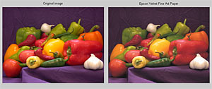
Click on image to see enlarged view.
Now we'll use the Epson Premium Glossy Photo Paper:
sRGB2glossy
= makecform('icc', sRGB_profile,
glossy_profile);
glossy2sRGB
= makecform('icc', glossy_profile,
sRGB_profile);
peppers_glossy
= applycform(peppers_sRGB, sRGB2glossy);
peppers_glossy_proof
= applycform(peppers_glossy, velvet2sRGB);
figure;
subplot(1,2,1);
imshow(peppers_sRGB);
title('Original
image'
subplot(1,2,2);
imshow(peppers_glossy_proof);
title('Epson
Premium Glossy Photo Paper'
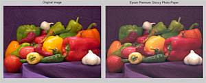
Click on image to see enlarged view.
Soft-proofing suggests that velvet paper image will have more saturation and "truer" colors (relative to the original) than the glossy paper. Note that this sort of proofing is valid only under certain lighting conditions, and doesn't show the effects of changing the paper angle or ink buildup (bronzing).
The functions used for soft-proofing can be used to simplify several image analysis tasks by converting images to L*a*b*. Some image processing and analysis operations, especially those involving color differences, are easier to perform in the L*a*b* color space than in RGB. L*a*b* is based on the opponent-color model of the human visual system. The L* channel is image luminosity, or brightness; the a* channel is a measure of red or green; and the b* channel contains blue-yellow information. Unlike RGB, L*a*b* is approximately perceptually uniform.
After converting the peppers image to L*a*b*, it can be segmented into redder or greener components:
sRGB2Lab = makecform('srgb2lab'
peppers_Lab
= applycform(peppers_sRGB, sRGB2Lab);
figure;
subplot(2,2,1);
imshow(peppers_sRGB);
title('RGB'
subplot(2,2,2);
imshow(peppers_Lab(:,:,1));
title('L
channel - Luminosity'
subplot(2,2,3);
imshow(peppers_Lab(:,:,2),[]);
title('a
channel - Red/Green'
subplot(2,2,4);
imshow(peppers_Lab(:,:,3),[]);
title('b
channel - Blue/Yellow'
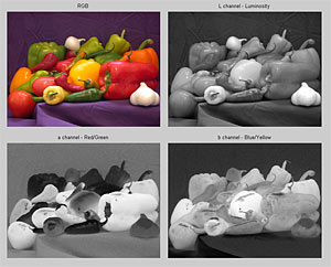
Click on image to see enlarged view.
The Image Processing Toolbox includes demos of segmentation using L*a*b*:
Color-Based Segmentation Using the L*a*b*
Color Space
Color-Based Segmentation Using K-Means
Clustering
Using the color difference metric ΔEa*b* in the L*a*b* color space, we gain empirical evidence that the velvet paper produced truer images than the glossy paper. For two images in the L*a*b* colorspace, the following function will approximate ΔEa*b*, which is the Euclidean distance between points in L*a*b*.
function dE =
deltaEab(image1Lab, image2Lab)
delta =
imabsdiff(image1Lab, image2Lab);
dE =
sqrt(double(delta(:,:,1) .^ 2 +
delta(:,:,2)
.^ 2 +
delta(:,:,3)
.^ 2));
Converting the "proof" images from sRGB to L*a*b* and then using the color difference measurement produces the error at each pixel in the image.
sRGB2Lab = makecform('srgb2lab'
peppers_Lab
= applycform(peppers_sRGB, sRGB2Lab);
peppers_velvet_Lab
= applycform(peppers_velvet_proof, sRGB2Lab);
peppers_glossy_Lab
= applycform(peppers_glossy_proof, sRGB2Lab);
dE_velvet
= deltaEab(peppers_Lab, peppers_velvet_Lab);
dE_glossy
= deltaEab(peppers_Lab, peppers_glossy_Lab);
figure;
subplot(1,2,1)
imshow(dE_velvet,[])
title(['Velvet:
Mean DeltaE_ = ' num2str(mean(dE_velvet(:)))])
subplot(1,2,2)
imshow(dE_glossy,[])
title(['Glossy:
Mean DeltaE_ = ' num2str(mean(dE_glossy(:)))])
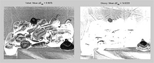
Click on image to see enlarged view.
Gamut mapping for glossy paper produces a larger overall error, as shown by the higher mean ΔEa*b* value and the brighter scaled error image.
Color management is an essential part of any imaging application where color fidelity matters. The Image Processing Toolbox and its support for ICC profiles provide a color-managed workflow for images in MATLAB, making it easy to simulate color changes among devices and fine-tune profiles for best results. In addition, the color transformation machinery provides a way to convert images into alternative color spaces, such as L*a*b* or XYZ, where they can be processed and analyzed more naturally.
|
Politica de confidentialitate | Termeni si conditii de utilizare |

Vizualizari: 2148
Importanta: ![]()
Termeni si conditii de utilizare | Contact
© SCRIGROUP 2025 . All rights reserved