| CATEGORII DOCUMENTE |
| Asp | Autocad | C | Dot net | Excel | Fox pro | Html | Java |
| Linux | Mathcad | Photoshop | Php | Sql | Visual studio | Windows | Xml |
Formatting Data with Excel
What you will learn from this lesson
With Excel 97 you will:
Use number formats.
Format using the Formatting toolbar.
Format numbers in cells.
Resize columns.
Use the AutoSum button (a
Format rows and columns.
Rotate text on your worksheet.
Customize the Formatting toolbar.
What you should do before you start this lesson
Start Excel 97.
Open a new workbook.
Exploring the lesson
When you enter numbers or text into any cell in Excel 97, you can format how the information is displayed. You can change the number to appear as a percentage or in any one of several formats.
Excel can display numbers in many ways. Any number can be entered as a plain number and then changed into another format.
Exploring number format
Trying different number formats
Click cell B2, type 123456, press enter, and then click B2 again.
On the Format menu, click Cells.
Note Another way to change format is to right-click the cell
that you want to format. On that shortcut menu, click Format Cells.
On the Number tab, choose Currency. In Decimal places,
click the down arrow until 0 appears, and then click OK.
Click B2, in the Formula Bar, type - in front of 12345, press enter, right-click cell B2, and click Format Cells.
On the Number tab, under Category, click Number, under Negative numbers, click 1234 in red, and click OK.
Close the workbook without saving changes.
Entering dates
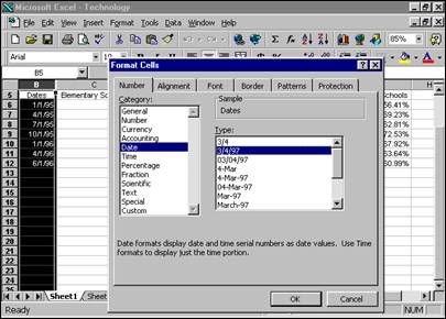
Displaying numbers as dates and formatting date cells
Open the Technology workbook you created earlier.
Right-click the B column header to select the dates and all of column B.
On the shortcut menu, click Format Cells.
On the Number tab, under Category, click Date.
Under Type, choose 3/4/97.
Click OK.
On the File menu, click Save.
Close the workbook.
Using Formatting toolbar buttons
In Excel 97, the Formatting toolbar buttons offer quick and easy ways to format cells.
Using the Formatting toolbar to change cell formats
Note Use the Merge and
Center button on the Formatting
toolbar.
Open a new
workbook.
![]()
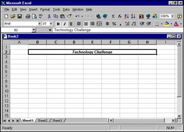
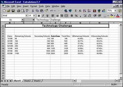
Click cell B2, and type Technology Challenge.
Press enter.
Click and drag cell B2 to cell H2.
Click cell H2. On the Formatting toolbar, click Merge and Center.
Select the words Technology Challenge.
Click the Italic button.
Click the Bold button.
Close the workbook without saving.
Formatting numbers in cells
Note Use these buttons to increase and decrease decimal
places.
Excel changes the
width of any cell as you enter the number. It automatically adjusts the width
to accommodate your numbers.
Formatting a cell with the Decrease Decimal and Increase Decimal buttons
Open a new workbook.
![]() In cell B4, enter 12345678999, and press enter.
In cell B4, enter 12345678999, and press enter.
Add a decimal point between 5 and 6, and press enter.
Click B4, and click the Decrease Decimal button twice.
Increase the number four times with the Increase Decimal button.
Close the workbook without saving.
 Resizing
columns
Resizing
columns
Now, your number is displayed as a percentage, but the cell extends across the entire screen. Use the Format menu to resize the column.
Resizing columns
On the Standard toolbar, click New.
Click cell D4, and type 12345.6666, and then press enter.
Right-click D4,and click Format Cells.
In the Number tab, click Number, click the up arrow in Decimal places to 6, and then click OK.
On the Format menu, select Column, and click Width.
In the Column Width box, type 24, and click OK.
In cell C6, repeat steps 1 through 3, but enter a width of 10, and see what happens to your number.
Position the pointer between the C and D columns until you see the double arrow, and then double-click.
Position the pointer between the D and E columns until you see the double arrow, and then click and drag until the width is 15.
Close the workbook without saving.
Note For an even faster way to use the AutoSum function, move
the pointer to the cell, and click alt+=.
Using the AutoSum
function
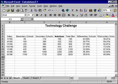
Excel 97 uses some math functions as buttons on the Standard toolbar. The AutoSum button is displayed as sigma, or a, and is used to calculate the sum of a range of numbers.
Totaling numbers
Open the Technology Report saved earlier.
Click the E column header, click the Insert menu, and then click Columns.
Click E6.
Click the AutoSum button on the Standard toolbar, and verify that the cells selected for summation are correct.
Press enter, and note the summation results in cell E6.
Click E6, and drag the fill handle to E12.
Close the workbook without saving your changes.
Note You can sum columns using the AutoSum button on the Standard toolbar or by using the Formula
bar as you did in the previous chapter.
Formatting rows and columns
Adjusting rows and columns so that the text within them is aligned left, centered, aligned right, or justified is quick and easy. Select the row or column, and use the buttons on the Formatting toolbar.
Note Use the Merge and
Center button to place text in the center of a single cell.
![]()
Centering rows
Centering the text in a title row makes the text easier to read.
Centering rows
In the Technology worksheet, select cells A1 through H1.
On the Formatting toolbar, click Merge and Center.
Click on row header 5 on the left margin to select the entire row.
On the Formatting toolbar, click the Center button to center all of the text in that row.
On the left margin, click row headers 6 through 12 to select all the cells, and click Center again on the Formatting toolbar.
Changing column alignment
Changing the alignment of columns makes a worksheet easier to read.
Aligning left
In the Technology worksheet, click column header C to select the entire column.
Click the Align Left button to left-align everything in the column.
Aligning right
In the Technology worksheet, click column header D to select the entire column.
Click the Align Right button to left-align everything in the column.
Try aligning several different cells and rows.
When you finish, close your workbook without saving.
How you can use what you learned
Now that you know how to sum data, calculate percentages, do simple calculation, and enter and edit text in your Excel 97 document, you are ready to start entering student seating charts or other student records. Use the workbook to record attendance, test scores, and assignments.
Extensions
Using Excel 97 you can create interesting charts to engage students, and you can challenge students to add charts to enhance their work and, at the same time, develop better creative-thinking skills.
Rotating text
Rotating the titles allows you to condense the title while keeping column headings readable. Rotating text on a worksheet is useful when you are recording grades and want to clearly label assignments. This feature allows you to format any cell on your worksheet. If you try to rotate merged cells, you may find that only the first letter will display.
Rotating text
Note Rotate column heads +90 degrees to read the text from
bottom to top; rotate the heads -90 degrees to read the text from top to
bottom.
Open the
Technology workbook.
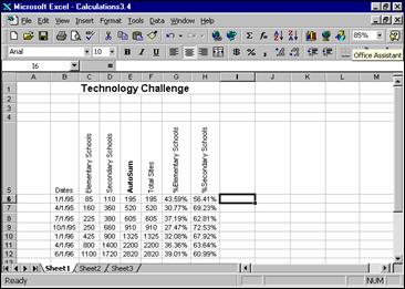
Click cells C5 through H5.
On the Format menu, click Cells.
On the Alignment tab, under Orientation, click and drag the Red Diamond to the vertical position.
![]()
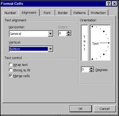
Click OK.
On the File menu, click Save As, and name the file Technology Challenge 1.2.
Click Save.
Close the workbook.
Customizing the Formatting toolbar
You can rotate text quickly and easily if you customize the Formatting toolbar by adding buttons for rotating text.
Customizing toolbars
Open a new workbook.
On the Tools menu, click Customize.
On the Commands tab, click Format.
Scroll to Rotate Text Up.
Click Rotate Text Up, and drag it to the right of the Merge and Center button on the toolbar.
Click Sheet2 to start a new worksheet.
Type Quizzes, Participation, and Exams in cells B5, C5, and D5, respectively.
Double-click between the headers of columns B and C, between C and D, and between D and E to center the text in the columns.
Select cells B5 through D5, and click the Rotate Text Up button.
Center the text in each of the columns.
Close the workbook without saving.
![]() Summarizing
what you learned
Summarizing
what you learned
In this chapter you have explored and practiced:
Using number formats.
Formatting with the Formatting toolbar.
Formatting numbers in cells.
Resizing columns.
Using the AutoSum button.
Formatting rows and columns.
Rotating text on your worksheet.
Customizing your Formatting toolbar.
|
Politica de confidentialitate | Termeni si conditii de utilizare |

Vizualizari: 1703
Importanta: ![]()
Termeni si conditii de utilizare | Contact
© SCRIGROUP 2025 . All rights reserved